Chapter 10 Comparing and Sorting the Bag of Words
We focus in this class on a particular sort of textual analysis: what are called bag of words approaches, and one of their most important subsets, the vector space model of texts.
The key feature of a bag of words approach to text analysis is that it ignores the order of words in the original text. These two sentences clearly mean different things:
- “Not I, said the blind man, as he picked up his hammer and saw.”
- “And I saw, said the not-blind man, as he picked up his hammer.”
But they consist of the same core set of words. The key question in working with this kind of data is the following: what do similarities like that mean? You’ll sometimes encounter a curmudgeon who proudly declares that “literature is not data” before stomping off. This is obviously true. And, as in the concordances we constructed last week or the digital humanities literature that relies more heavily on tools from natural language processing, there are many ways to bring some of the syntactic elements of language into play.
But bag-of-words approaches have their own set of advantages: they make it possible to apply a diverse set of tools and approaches from throughout statistics, machine learning, and data visualization to texts in ways that can often reveal surprising insights. In fact, methods developed to work with non-textual data can often be fruitfully applied to textual data, and methods primarily used on textual data can be used on sources that are not texts. You may have an individual project using humanities data that is not textual. For example, we saw last week how Zipf’s law of word distributions applies to our city sizes dataset just as it applies to word counts. Almost all of the methods we’ll be looking at can be applied as easily, and sometimes as usefully, to other forms of humanities data. (Streets in a city, soldiers in an army, or bibliographic data.) But to do so requires transforming them into a useful model.
10.1 Three metrics
10.1.1 Metrics
This section is one of the high points of the math in this course, because we’re talking about
three metrics. By metric I mean a score that represents something useful about a word. So far,
we’ve used a number of basic properties inside ‘summarize’ and ‘mutate’ calls, but you’ve
generally known what they do from the name: mean, median, sum, min, and so on.
frequency, which we’ve looked at a bit lately, is slightly less transparent, but still easily understood;
for words, it means the rate at which it’s used.
For working with counts, these aren’t always sufficient, and you need to resort to some specialized measures. This chapter introduces three of the most basic ones in digital humanities research.
- TF-IDF: for search and OK for comparison
- Pointwise Mutual information: for comparing incidence rates.
- Dunning Log-likelihood: for making statistically valid comparisons.
TF-IDF is a more document-specific approach, that comes from the world of information retrieval; PMI comes more from the information science side of the world.
10.1.2 TF-IDF: let’s build a search engine
Humanists use search engines constantly, but we don’t know how they work. You might think that’s OK: I drive a car with a variable transmission, but have absolutely no idea how it works. But the way that what you read is selected is more than a technical matter for a researcher; it’s at the core of the research enterprise. So to understand how bag-of-words approaches work, we’ll start by looking at one metric that is frequently used in search engines, something called TF-IDF.
A core problem of information retrieval is that, especially with multiword phrases, people don’t
necessarily type what they want. They might, for example,
search state of the union addresses for the words iraq america war. One of these words–“Iraq”–
is much less common than the other two; but if you placed both into a search, you’d probably be overwhelmed
by results for ‘war’ and America.
One solution might simply to be to say: rare words are the most informative, so we should overweight them. But by how much? And how should we define rareness?
There are several possible answers for this. The answer to this is based in an intuition related to Zipf’s law, about how heavily words are clustered in documents.
Here’s how to think about it. The most common words in State of the Union addresses are words like
‘of’, ‘by’, and ‘the’ that appear in virtually every State of the Union.
The rarest words probably only appear in a single document. But what happens if we compare those
two distributions to each other? We can use the n() function to count both words and documents, and
make a comparison between the two.
To best see how this works, it’s good to have more than the 200 State of the Union addresses, so we’re going to break up each address into 2,000 word chunks, giving us about 1,000 documents of roughly equal length. The code below breaks this up into four steps to make it clearer what’s going on:
library(tidytext)
library(HumanitiesDataAnalysis)
library(tidyverse)

# Add 2000-word chunks
allSOTUs = get_recent_SOTUs(1789) %>%
  group_by(filename) %>%
  add_chunks(chunk_length = 2000)
## Joining, by = "year"chunked_SOTU = allSOTUs %>%
group_by(filename, chunk) %>%
count(word) %>%
mutate(total_documents = n_groups(.))
# For each word, get the total occurrences *and* the number
# of documents it appears in.
word_statistics = chunked_SOTU %>%
group_by(total_documents, word) %>%
summarize(documents = n(), n = sum(n)) %>%
mutate(document_share = documents / total_documents, word_share = n / sum(n)) %>%
arrange(-n) %>%
mutate(expected_docs = (1 - (1 - 1 / total_documents)^n))The red line shows how many documents each word would show up in if words were distributed randomly. They aren’t; words show up in chunky patterns. A paragraph that says “gold” once is more likely to use the word “gold” again than one that says “congress.”
This chunkiness, crucially, is something that differs between words. The word “becoming” doesn’t cluster within paragraphs; the word “soviet” does. TF-IDF exploits this pattern.
library(ggrepel)

word_statistics %>%
  ungroup() %>%
  ggplot() + aes(x = n, y = document_share, label = word) +
  geom_point(alpha = 0.2) +
  scale_y_log10("Percent of documents", labels = scales::percent) +
  scale_x_log10("Total Occurrences", labels = scales::comma, breaks = 10^(0:5)) +
  geom_line(aes(y = expected_docs), color = "red", lwd = 2, alpha = .33) +
  geom_label_repel(data = word_statistics %>% filter(word %in% c("gold", "the", "becoming", "soviet", "america", "congress", "these", "every", "iraq")), fill = "#FFFFFFAA") +
  labs(title = "Word Frequency and document share", subtitle = "The more common a word is, the more documents it appears in...\n but some words are in just a few documents")
Rather than plotting on a log scale, TF-IDF uses a statistic called the ‘inverse document frequence.’ The alteration to the plot above is extremely minor. First, it calculates the inverse of the document frequency, so that a word appearing in one of a hundred documents gets a score of 100, not of 0.01; and then it takes the logarithm of this number.
This logarithm is an extremely useful weight. Since log(1) == 0, the weights for words that appear in every single document
will be zero. That means that extremely common phrases (in this set, those much more common than ‘congress’) will be thrown out altogether.
word_statistics %>%
  mutate(IDF = log(total_documents / documents)) %>%
  ggplot() +
  geom_point(aes(x = n, y = IDF)) +
  scale_x_log10() + labs(title = "IDF weights are just the inverse of log-scaled documents percentages")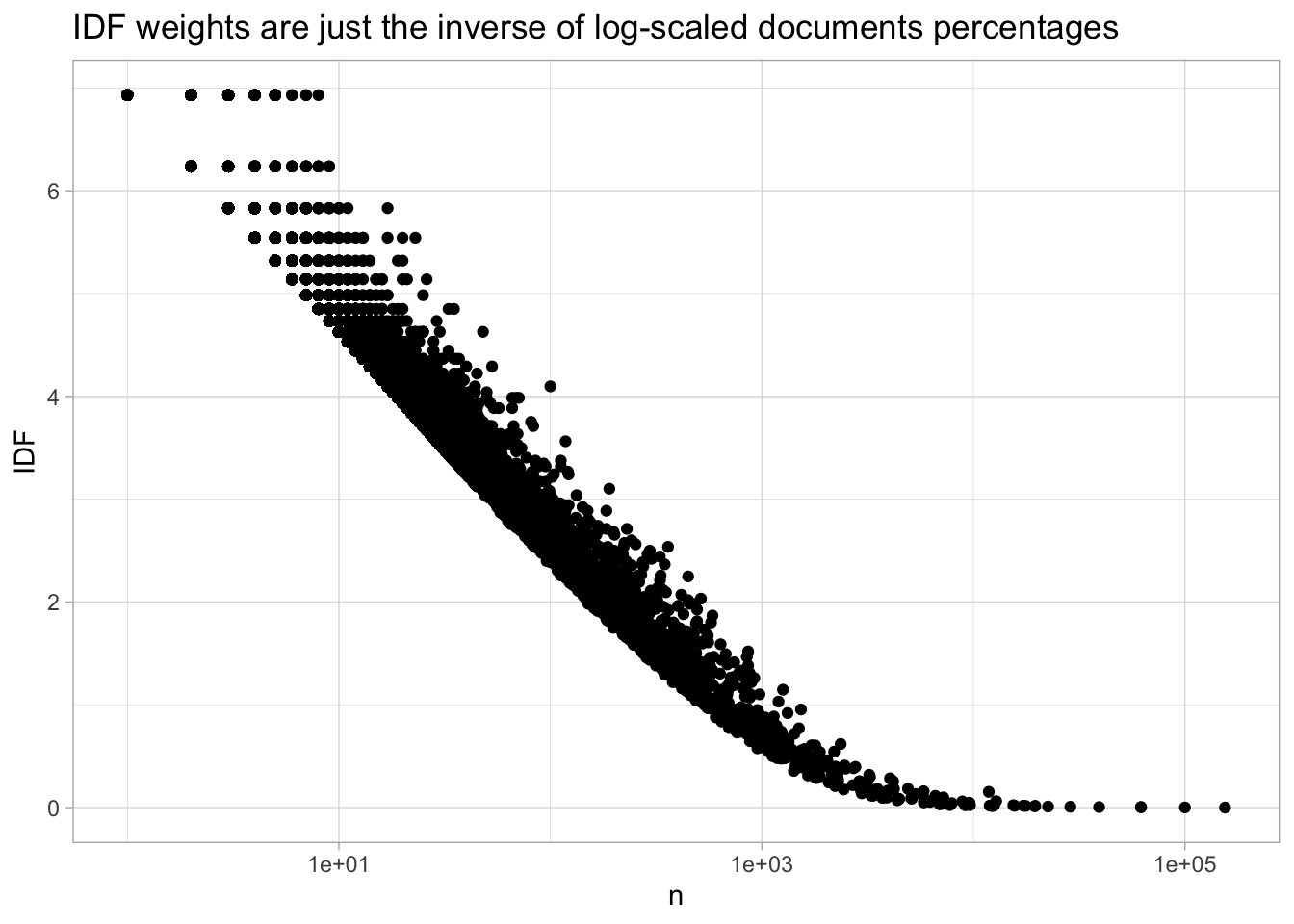
Finally, these IDF weights are multiplied by the term frequency.
tf_idf = word_statistics %>%
  mutate(IDF = log(total_documents / documents)) %>%
  ungroup %>%
  select(word, IDF) %>%
  inner_join(allSOTUs %>% count(filename, chunk, word)) %>%
  group_by(filename, chunk) %>%
  mutate(tf = n / sum(n)) %>%
  mutate(tf_idf = tf * IDF)
## Joining, by = "word"This is one of the functions bundled into the module I’ve shared with you. You can run TF-IDF on any set of documents to see the distinguishing features. For instance, if we group by ‘president,’ we can see the terms that most distinguish each president.
So–say that we want to do a search for “Iraq”, “America”, and “War”.
One way to build our own search engine is to make a table of those words,
and join it to our already-created tf_idf weights. One of our tried-and-true
summary operations can count up the scores.
search = tibble(word = c("iraq", "iraqis", "america"))

doc_scores = tf_idf %>%
    group_by(chunk, filename) %>%
    filter(sum(n) > 1500) %>%
    inner_join(search) %>%
    group_by(chunk, filename) %>%
    summarize(score = sum(tf_idf), count = sum(n)) %>%
    arrange(-score)
## Joining, by = "word"Here are the first fifty words of the chunks that most strongly match our query.
tf_idf %>%
  filter(word %in% c("iraq", "iraqis", "america")) %>%
  group_by(filename, chunk) %>%
  summarize(score = sum(tf_idf)) %>%
  arrange(-score) %>%
  head(3) %>%
  inner_join(allSOTUs) %>%
  slice(1:50) %>%
  summarize(score = score[1], text = str_c(word, collapse = " ")) %>%
  pull(text)
## Joining, by = c("filename", "chunk")## [1] "world last sunday across iraq often at great risk millions of citizens went to the polls and elected 275 men and women to represent them in a new transitional national assembly a young woman in baghdad told of waking to the sound of mortar fire on election day and wondering"
## [2] "by extending the frontiers of medicine without the destruction of human life so we're expanding funding for this type of ethical medical research and as we explore promising avenues of research we must also ensure that all life is treated with the dignity it deserves and so i call on"
## [3] "i have ever been that the state of our union is strong thank you god bless you god bless the united states of america"allSOTUs %>%
group_by(president) %>% # <- Define documents
count(word) %>%
summarize_tf_idf(word, n) %>% # <- calculate scores for each word/document pair
group_by(president) %>%
arrange(-.tf_idf) %>%
filter(str_detect(word, "[a-z]")) %>% # The most informative word for many presidents is a year.
slice(1)## Joining, by = "word"10.1.3 Pointwise mutual information
TF-IDF is primarily designed for document retrieval; it has been used quite a bit, though, as a way to extract distinguishing words.
TF-IDF, though, is not a foolproof way to compare documents. It works well when the number of documents is relatively large (at least a couple dozen, say); but what if there are just 2 classes of documents that you want to compare? Or what if the documents are radically different sizes?
One very basic answer is a metric with an intimidating name, but a rather simple definition, called “pointwise mutual information.” I think of pointwise mutual information as simply a highfalutin way of something I think of as the “observed over expected ratio.” What it means, simply, is how often an event occurs compared to how often you’d expect it to occur. We have already encountered a version of this statistic earlier: when we looked at the interactions of hair color and skin color among sailors in the New Bedford Customs Office dataset.
In fact, you may often find yourself coding a version of pointwise mutual information just in the course of exploring data.
PMI looks at the overall counts of documents and words to see how frequent each are: and then it estimates an expected rate of usage of each word based on how often it appears overall. For instance, if all presidents use the pronoun “I” at a rate of 1% of all words, you’d expect Barack Obama to also use it at that same rate. If he uses it at 1.5% instead, you could say that it’s 50% more common than expected.
Although this is built into the package functions, it’s simple enough to implement directly using functions we understand that it’s worth actually looking at as code.
president_counts = allSOTUs %>%
  inner_join(presidents) %>%
  filter(year > 1981) %>%
  group_by(president, word) %>%
  summarize(count = n()) %>%
  ungroup()
## Joining, by = c("year", "president", "party", "sotu_type")pmi_scores = president_counts %>%
## What's the total number of words?
mutate(total_words = sum(count)) %>%
## What share of all words does the word have?
group_by(word) %>%
mutate(word_share = sum(count) / total_words) %>%
# Define our documents to be all the works of a president.
group_by(president) %>%
mutate(president_word_share = count / sum(count)) %>%
## You would expect each word to occur as a percentage of the total defined
## by the document and the president.
mutate(ratio = president_word_share / word_share)
pmi_scores %>%
filter(word %in% c("i", "will", "make", "america", "great", "again")) %>%
ggplot() +
geom_point(aes(y = president, x = ratio)) +
facet_wrap(~word) +
scale_x_continuous(labels = scales::percent)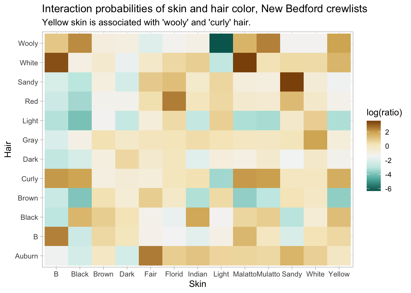
The visual problem is that we’re plotting a ratio on a linear scale on the x axis. But in reality, it often makes more sense to cast ratios in terms of a logarithmic scale, just as we did with word count ratios. If something is half as common in Barack Obama’s, that should be as far from “100%” as something that is twice as common.
Usually, we’d represent this by just using a log-transformation on the x-axis; but the log-transformation is so fundamental
in this particular case that it’s actually built into the definition of pointwise mutual information. Formally, PMI is defined
as the logarithm of the ratio defined above. Since log(1) is zero, a negative PMI means that some combination is
less common than you might expect, and a positive one that it’s more common than you’d expect. It’s up to you to decide if you’re
working in a context where calling something ‘PMI’ and indicating the units as bits; or if you’re writing for a humanities
audience and it make more sense to explicitly call this the ‘observed-expected ratio.’
If you’re plotting things, though, you can split the difference by using a logarithmic scale on the observed-expected value.
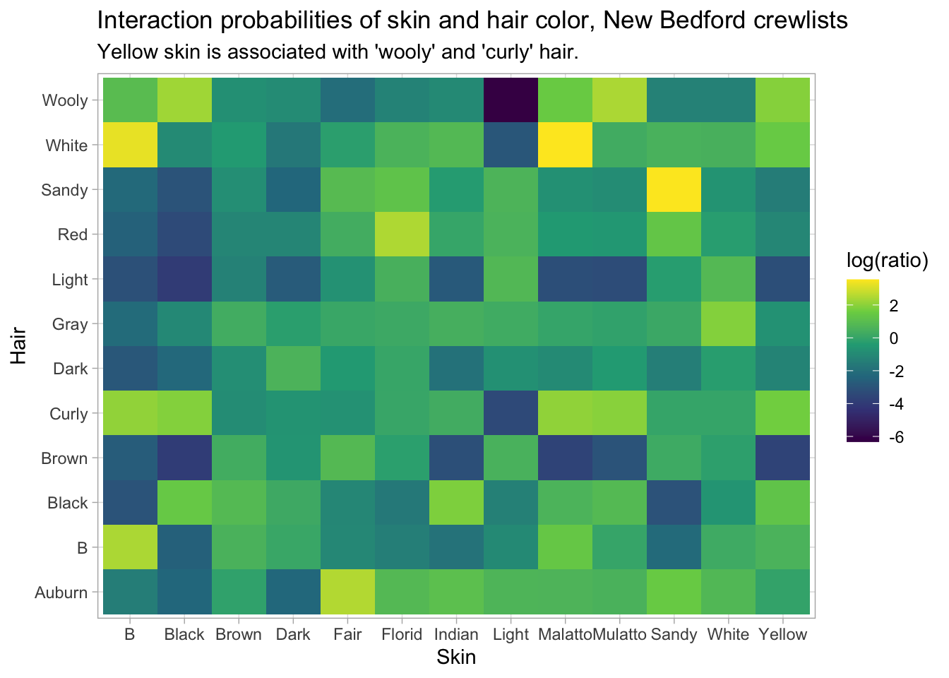
You can use PMI across wordcount matrices, but it also works on anything else where you can imagine an expected share of counts. We already talked about the observed and expected interactions of skin color and hair color in shipping datasets.
crews %>%
  count(Skin, Hair) %>%
  filter(!is.na(Skin), !is.na(Hair)) %>%
  # Add '0' counts where data is missing--e.g., no one is listed
  # has having light skin and wooly hair.
  complete(Skin, Hair, fill = list(n = 0)) %>%
  add_count(Skin, wt = n, name = "skin_count") %>%
  add_count(Hair, wt = n, name = "hair_count") %>%
  add_count(wt = n, name = "total_count") %>%
  mutate(expected = skin_count / total_count * hair_count / total_count * total_count) %>%
  filter(skin_count > 100, hair_count > 100) %>%
  mutate(ratio = ifelse(n == 0, 1, n) / expected) %>%
  arrange(-expected) %>%
  ggplot() +
  geom_tile(aes(x = Skin, y = Hair, fill = log(ratio))) + scale_fill_viridis_c() + labs(
    title = "Interaction probabilities of skin and hair color, New Bedford crewlists",
    subtitle = "Yellow skin is associated with 'wooly' and 'curly' hair."
  )
You can also look at word counts in a specific context: for instance, what words appear together more than you’d expect given their mutual rates of occurence? Using the lag function, we can build a list of bigrams and create a count table of how many times any two words appear together. Since each of these are events we can imagine a probability for, we can calculate PMI scores to see what words appear together in State of the Union addresses.
Some of these are obvious (‘per cent.’) But others are a little more interesting.
bigrams = allSOTUs %>%
  ungroup() %>%
  mutate(word2 = lead(word, 1)) %>%
  # Count the occurrences of each bigram
  count(word, word2) %>%
  ungroup() %>%
  add_count(word2, wt = n, name = "word2_n") %>%
  add_count(word, wt = n, name = "word_n") %>%
  add_count(wt = n, name = "total_words") %>%
  mutate(expected = word_n / total_words * word2_n / total_words * total_words) %>%
  filter(n > 100) %>%
  mutate(ratio = n / expected, pmi = log(ratio)) %>%
  arrange(-ratio)

bigrams %>%
  select(word, word2, pmi) %>%
  head(10)
10.1.4 Dunning Log-Likelihood.
While this kind of metric seems to work well for common words, it starts to break down when you get into rarer areas. If you sort by negative PMI on the president-wordcount matrix (try this on your own to see what it looks like), all the highest scores are for words used only by the president who spoke the fewest words in the corpus.
These kinds of errors–low-frequency words showing up everywhere on a list–are often a sign that you need to think statistically.
One useful comparison metric for wordcounts (and anyother count information) is a test known as Dunning log-likelihood. It expresses not just a descriptive statement about relative rates of a word, but a statistical statement about the chances that so big a gap might occur randomly. It bears a very close relationship to log-likelihood. In addition to calculating the observed-expected ratio for a word occurring in a corpus, you also calculate the observed-expected ratio for the word in all the works not in that corpus.
The sum of these quantities gives you a statistical score that represents a quantity of certainty that a different in texts isn’t by chance. Here’s some pseudo-code if you’re interested:
counts = allSOTUs %>%
  ungroup() %>%
  mutate(word2 = lead(word, 1)) %>%
  # Count the occurrences of each bigram
  count(word, word2) %>%
  group_by(word) %>%
  summarize_pmi(word2, n)

dun_test = counts %>%
  group_by(word2) %>%
  mutate(
    .count = count,
    global_occurrences = sum(.count) - .count,
    global_expected = ((sum(.doc_total) - .doc_total) * .word_share),
    pmi_for_everything_else = global_occurrences * log(global_occurrences / global_expected),
    scaled = .count * .pmi,
    dunning = 2 * (pmi_for_everything_else + scaled),
    signed_dunning = dunning * ifelse(.pmi < 0, -1, 1)
  )

dun_test %>% arrange(-signed_dunning) %>% head(5) %>% select(word, word2, .pmi, dunning)
PMI tends to focus on extremely rare words. One way to think about this is in terms of how many times more often a word appears than you’d expect. Suppose we compare just two parties since 1948, Republicans and Democrats: suppose I say my goal to answer this question:
What words appear the most times more in Democratic Speeches and Republican ones, and vice versa?
There’s already an ambiguity here: what does “times more” mean? In plain English, this can mean two completely different things. Say R and D speeches are exactly the same overall length (I chose 1948 because both parties have about 190,000 words apiece). Suppose further “allotment” (to take a nice, rare, American history word) appears 6 times in R speeches and 12 times in D speeches. Do we want to say that it appears two times more (ie, use multiplication), or six more times (use addition)?
It turns out that neither of these simple operations works all that well. PMI is, roughly, the same as multiplication. In the abstract, multiplication probably sounds more appealing; but it actually catches extremely rare words. In our example set, here are the top words that distinguish R from D by multiplication, by occurences in R divided by occurrences in D. For example, “lobbyists” appears 20x more often in Democratic speeches than Republican ones.
presidents_over = allSOTUs %>%
  ungroup %>% filter(year > 1948) %>%
  filter(party %in% c("Republican", "Democratic")) %>%
  count(party, word) %>%
  pivot_wider(values_from= n, names_from = c(party), values_fill = c(n = 1)) %>%
  mutate(multiplication = `Democratic` / `Republican`,
         addition = `Democratic` - `Republican`)

presidents_over %>%
  arrange(-multiplication) %>%
  select(word, multiplication, Democratic, Republican) %>%
  head(5)
By number of times, the Democrats are distinguished by stopwords–to, we, and ‘our’. We can assume that ‘the’ is probably a Republican word.
Is there any way to find words that are interesting on both counts?
I find it helpful to do this visually. Suppose we make a graph. We’ll put the addition score on the X axis, and the multiplication one on the Y axis, and make them both on a logarithmic scale. Every dot represents a word, as it scores on both of these things. Where do the words we’re talking about fall? It turns out they form two very distinct clusters: but there’s really a tradeoff here.
presidents_over %>%
  filter(addition > 0) %>%
  ggplot() + geom_point(alpha = 0.2) +
  aes(x=addition, y = multiplication, label=word) +
  scale_x_log10("Times more by multiplication") +
  scale_y_log10("Times more by addition") +
  geom_label_repel(data = presidents_over %>% filter(rank(-addition) < 10 | rank(-multiplication) < 10)) +
  labs(main="The 10 words most distinguishing of Democratic vs. Republican speeches", subtitle = "By 'times more' in addition and multiplication")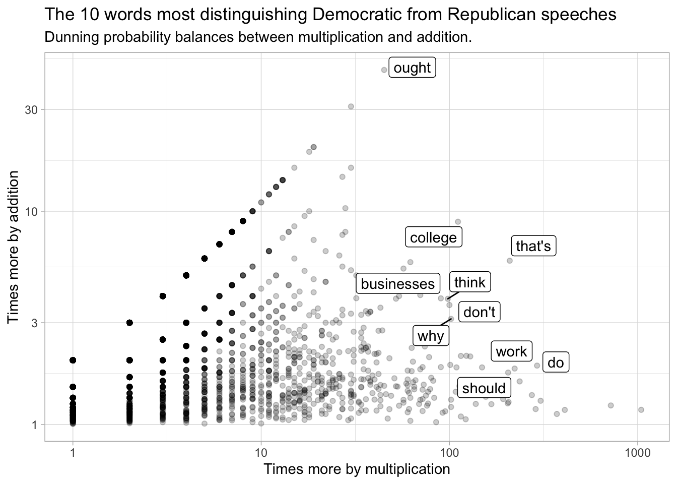
Dunning’s log-likelihood score provide a way of balancing between these two views. We use them the same way as
the other summarize functions; by first grouping by documents (here ‘party’) and calling summarize_llr(word, n)
where word is the quantity we’re counting and n is the count of fields.
If we redo our plot with the top Dunning scores, you can see that the top 15 words pulled out lie evenly distributed between our two metrics; Democratic language is now more clearly distinguished by its use of–say–the word ‘college.’
dunning_ps =  allSOTUs %>%
  ungroup %>% filter(year > 1948) %>%
  filter(party %in% c("Republican", "Democratic")) %>%
  count(party, word) %>%
  group_by(party) %>%
  summarize_llr(word, n) %>% arrange(-.dunning_llr) %>%
  filter(party=="Democratic")

presidents_over %>%
  filter(addition > 0) %>%
  ggplot() + geom_point(alpha = 0.2) +
  aes(x=addition, y = multiplication, label=word) +
  scale_x_log10("Times more by multiplication") +
  scale_y_log10("Times more by addition") +
  geom_label_repel(data = presidents_over %>% inner_join(dunning_ps %>% head(10))) +
  labs(title="The 10 words most distinguishing Democratic from Republican speeches", subtitle = "Dunning probability balances between multiplication and addition.")
## Joining, by = "word"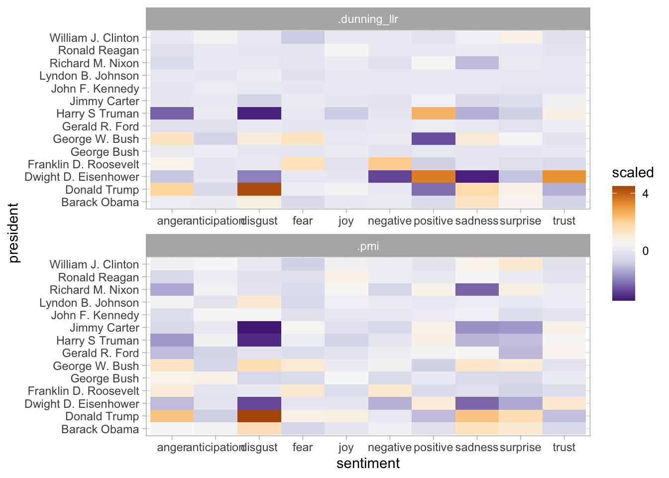
We can also do Dunning comparisons against a full corpus with multiple groups. Here, for example, is a way of thinking about the distinguishing words of multiple presidents State of the Union addresses.
dunning_scores = allSOTUs %>%
  group_by(president) %>%
  filter(year > 1980) %>%
  count(word) %>%
  summarize_llr(word, n)

dunning_scores %>%
  arrange(-.dunning_llr) %>%
  group_by(president) %>%
  slice(1:15) %>%
  ggplot() +
  geom_bar(aes(x = reorder(word, .dunning_llr), y = .dunning_llr), stat = "identity") +
  coord_flip() +
  facet_wrap(~president, scales = "free_y") +
  labs("The statistically most distinctive words in each modern president's state of the Union addresses.")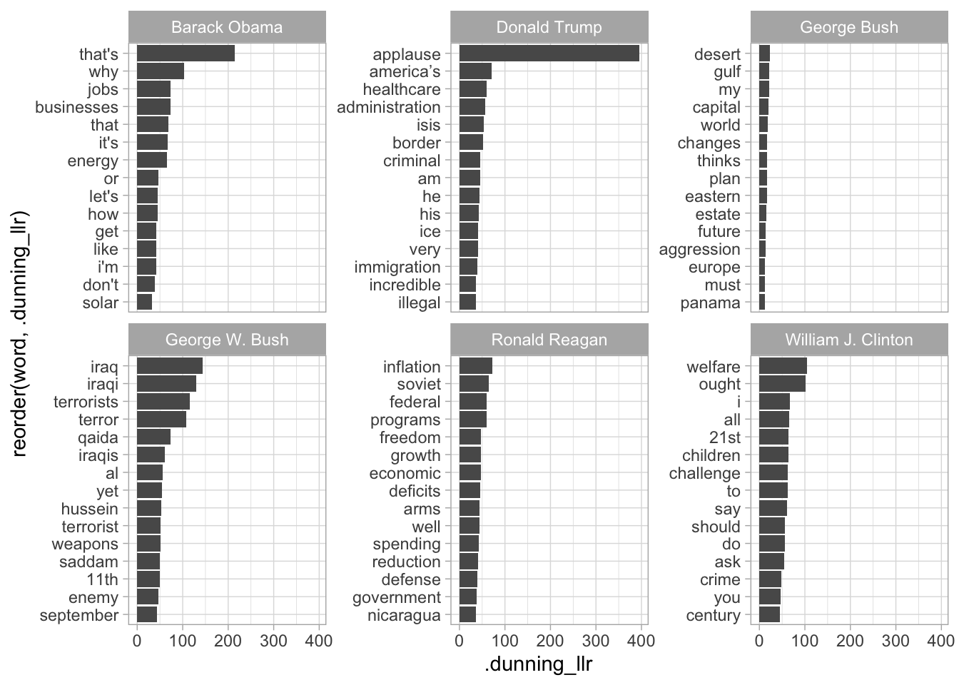
These are not prohibitive problems; especially if you find some way to eliminate uncommon words. One way to do this, of course, is simply to eliminate words below a certain threshold. But there are more interesting ways. Just as we’ve been talking about how the definition of ‘document’ is flexible, the definition of “word” can be too. You could use stemming or one of the approaches discussed in the “Bag of Words” chapter. Or you can use merges to count something different than words.
For example, we can look at PMI across not words but sentiments. Here we’ll use a rather complicated list published in Saif M. Mohammad and Peter Turney. (2013), “Crowdsourcing a Word-Emotion Association Lexicon.” Computational Intelligence, 29(3): 436-465 that gives not just positive and negative, but a variety of different views. Essentially this is sort of like looking at words in greater numbers.
In this case, both the PMI and Dunning scores give comparable results, but the use of statistical certainty
means that some things–like whether Jimmy Carter uses language of ‘disgust’–are quite suppressed.
Here I calculate scores separately, and then use a pivot_longer operation to pull them together.
(Note that there’s one new function here: scale is a function that brings multiple
variables into a comparable scale–standard deviations from the mean–so that you can compare them.
You’ll sometimes see references to ‘z-score’ in social science literature. That’s what
scale does here.
sentiments = tidytext::get_sentiments("nrc")

pmi_matrix = allSOTUs %>%
  filter(year > 1934) %>%
  filter(word != "applause") %>%
  filter(word != "congress") %>%
  inner_join(sentiments) %>%
  group_by(president, sentiment) %>%
  summarize(count = n()) %>%
  group_by(president) %>%
  summarize_pmi(sentiment, count)
## Joining, by = "word"dunning_matrix = allSOTUs %>%
filter(year > 1934) %>%
filter(word != "applause") %>%
filter(word != "congress") %>%
inner_join(sentiments) %>%
group_by(president, sentiment) %>%
summarize(count = n()) %>%
group_by(president) %>%
summarize_llr(sentiment, count)## Joining, by = "word"pmi_matrix %>%
inner_join(dunning_matrix) %>%
select(president, sentiment, .dunning_llr, .pmi) %>%
pivot_longer(c(.pmi, .dunning_llr), names_to = "metric", values_to = "value") %>%
group_by(metric) %>%
mutate(scaled = scale(value)) %>%
ggplot() +
geom_tile(aes(x = president, y = sentiment, fill = scaled)) +
scale_fill_distiller(palette = "PuOr", type='div', breaks = c(-4, 0, 4)) +
coord_flip() +
facet_wrap(~metric, ncol = 1, scales = "free") +
labs("")## Joining, by = c("president", "sentiment")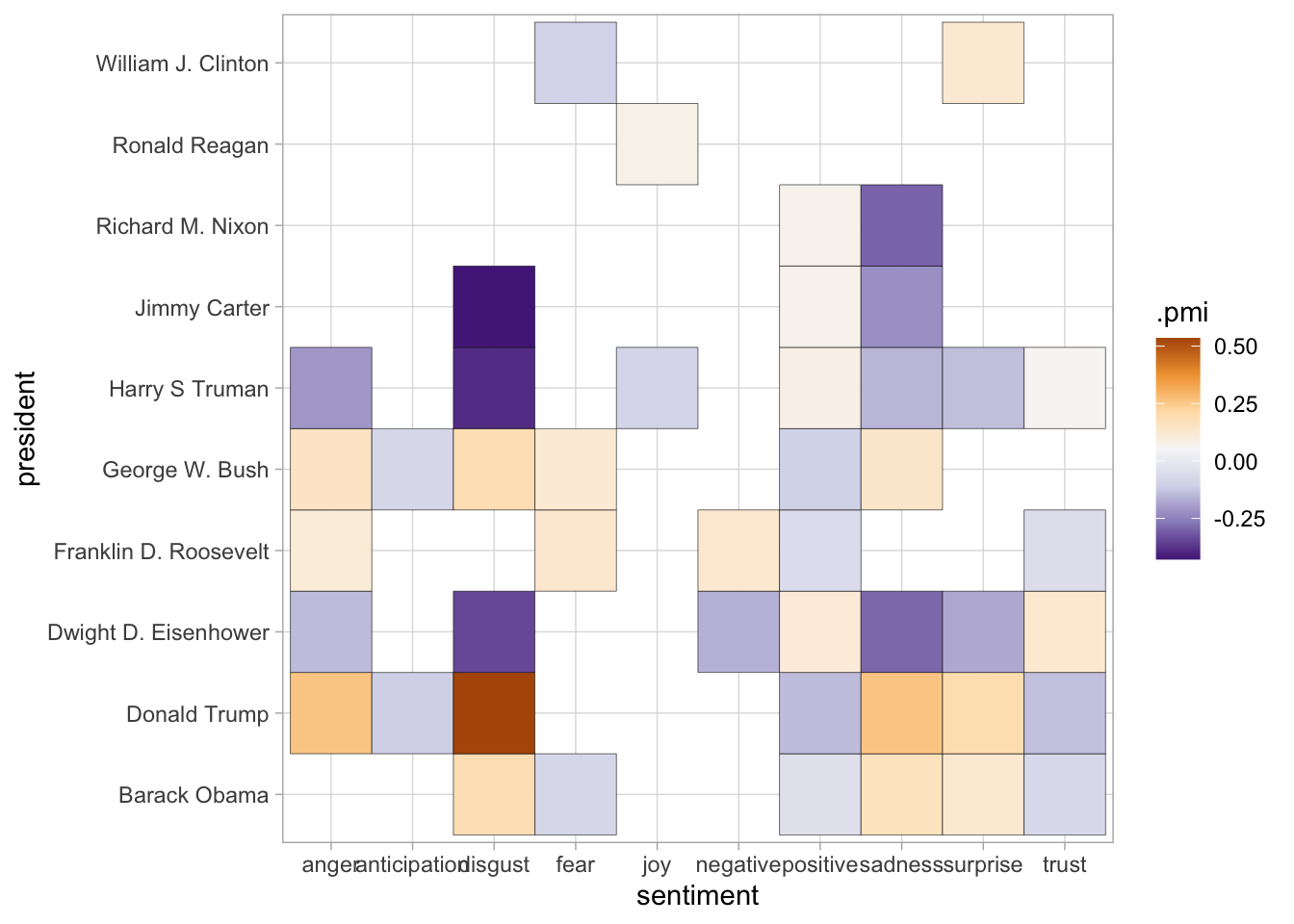
Another reason to use Dunning scores is that they offer a test of statistical significance; if you or your readers are worried about mistaking a random variation for a significance one, you should be sure to run them. Conversely, the reason to use PMI rather than log-likelihood is that it is actually a metric of magnitude, which is often closer to the phenomenon actually being described; especially if you use the actual observed/expected counts, rather that the log transformation.
So one strategy that can be useful is to use a significance test directly on the Dunning values.
The function included in this package includes a column in the return value called (.dunning_significance);
that indicates whether or not the difference at that location is statistically significant or not.
(The calculations for doing this are slightly more complicated; they involve looking up the actual Dunning score in
and translating it to a probability, and then applying a method called the Holm-Sidak correction for multiple comparisons
because the raw probabilities don’t account for the fact that with wordcounts we make hundreds of comparisons.)
The chart below shows just the PMI values, but drops out all entries for which the Dunning scores indicate no statistical significance.
pmi_matrix %>%
  inner_join(dunning_matrix) %>%
  filter(.dunning_significance) %>%
  select(president, sentiment, .dunning_llr, .pmi) %>%
  ggplot() +
  geom_tile(aes(x = president, y = sentiment, fill = .pmi), color="black") +
  scale_fill_distiller(palette = "PuOr", type='div') +
  coord_flip() +
  labs("")
## Joining, by = c("president", "sentiment")
10.2 The term-document matrix
You can do a lot with purely tidy data, but another useful feature is something known as the “term-document matrix.” This is a data structure extremely similar to the ones that we have been building so far: in it, each row refers to a document, and each column describes a word.
This is not “tidy data” in Wickham’s sense, so it can be easily generated from it using the pivot_wider function in his tidyr package. Let’s investigate by looking at some state of the Union Addresses.
Here we re-use the read_tokens function we wrote in the previous chapter.
## Joining, by = "year"With state of the union addresses, the most obvious definition of a document is a speech: we have that here in the frame “year”.
We also want to know how many times each word is used. You know how to do that: through a group_by and summarize function.
counts = allSOTUs %>%
  mutate(word = tolower(word)) %>%
  group_by(year, word) %>%
  summarize(count = n()) %>%
  ungroup()

counts %>% head(30)
In a term-document matrix, the terms are the column names, and the values are the counts. To make this into a term-document matrix, we simply have to spread out the terms along these lines.
td_matrix = counts %>%
  filter(word != "") %>%
  spread(word, count, fill = 0)

counts = counts %>%
  filter(word != "")
Usually, we’ve looked at data with many rows and few columns. Now we have one that is 229 columns rows by 29,000 columns. Those 10,000 columns are the distinct rows.
Later, we’ll work with these huge matrices. But for now, let’s set up a filter to make the frame a little more manageable.
Note that I’m also renaming the ‘year’ column to ‘.year’ with a period.
That’s because ‘year’ is a word as well as a column, and in the wide form we can’t have columns capturing both meanings.
td_matrix = counts %>%
  group_by(word) %>%
  rename(.year = year) %>%
  filter(sum(count) > 100) %>%
  ungroup() %>%
  pivot_wider(names_from = word, values_from = count, values_fill = c("count" = 0))

# This shows only the first few of about 30 columns.
td_matrix %>%
  head(30) %>%
  select(.year:adequate)
Consider some slices of the term-document matrix. These look sort of like what we’ve been doing before.
ggplot(td_matrix) +
  aes(x = the, y = and, color = .year) +
  geom_point() +
  scale_color_viridis_c() +
  scale_x_log10() +
  scale_y_log10()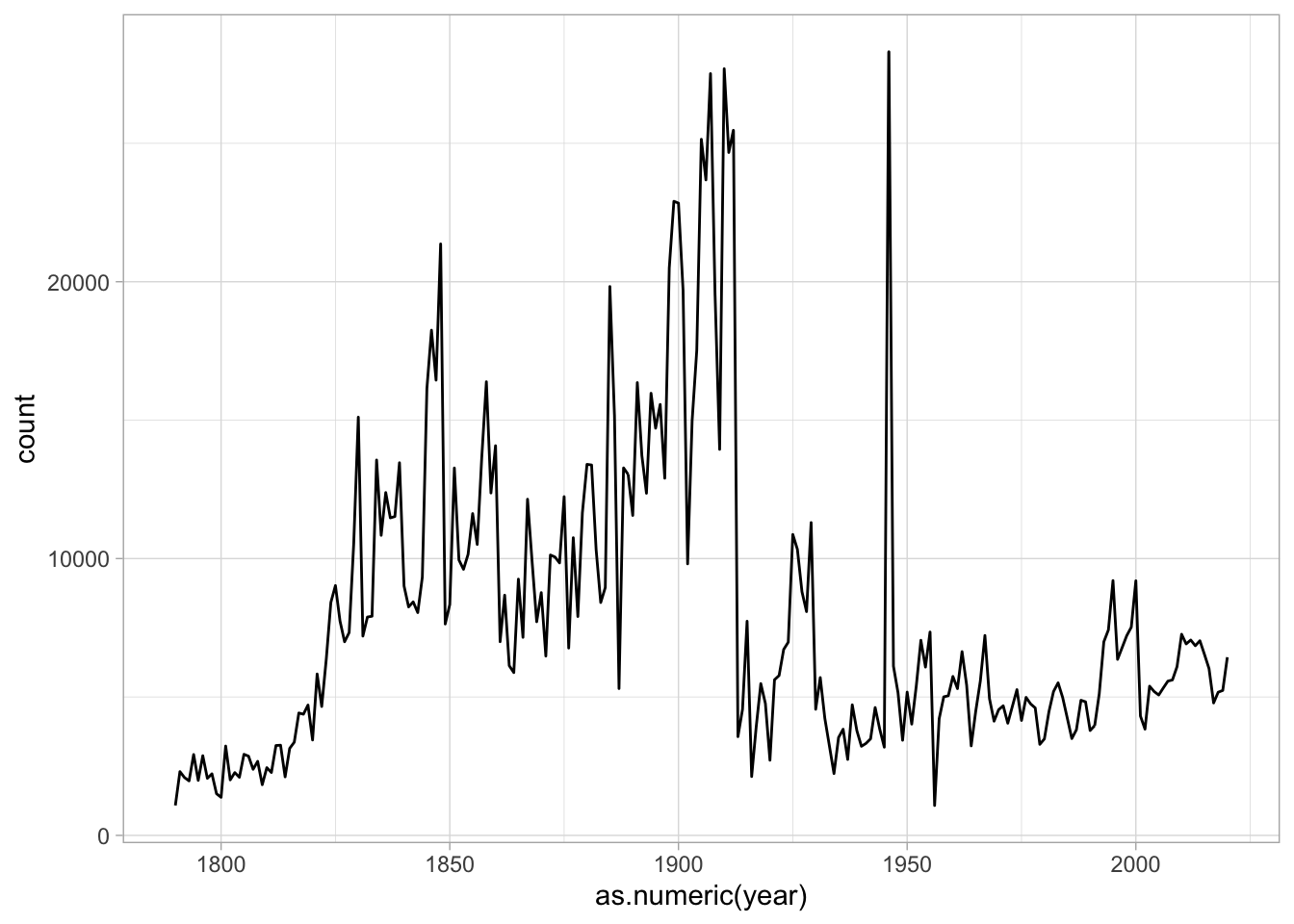
With this sort of data, it’s more useful to compare against a different set of texts.
parties = presidents %>% rename_all(. %>% str_c(".", .))
td_matrix = td_matrix %>% inner_join(parties)
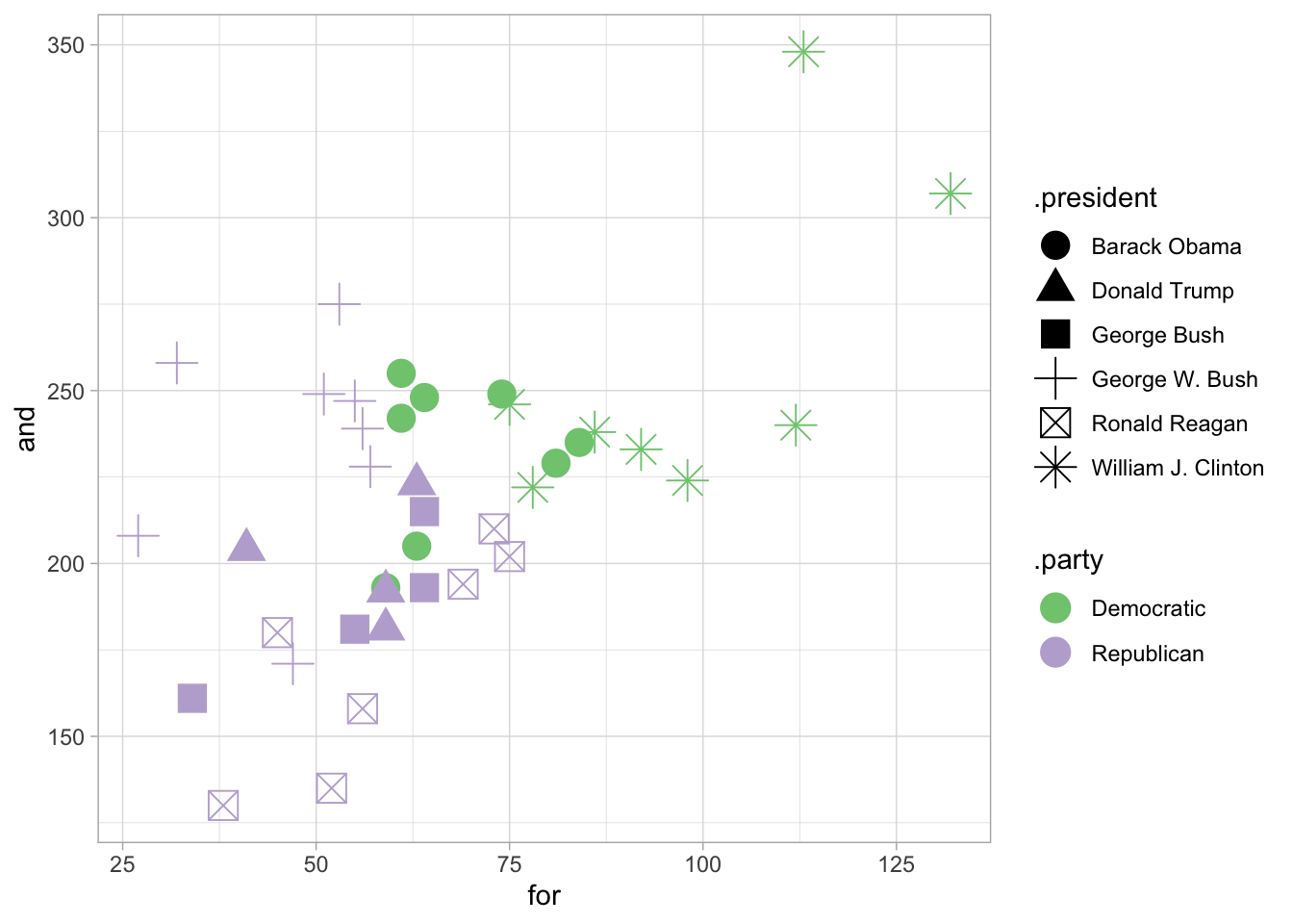
## Joining, by = ".year"Here’s an ggplot of usage of “and” and “for” in State of the Union addresses since 1981
td_matrix %>%
  filter(.year > 1981) %>%
  ggplot() +
  aes(x = `for`, y = and, pch = .president, color = .party) +
  geom_point(size = 5) +
  scale_color_brewer(type = "qual")
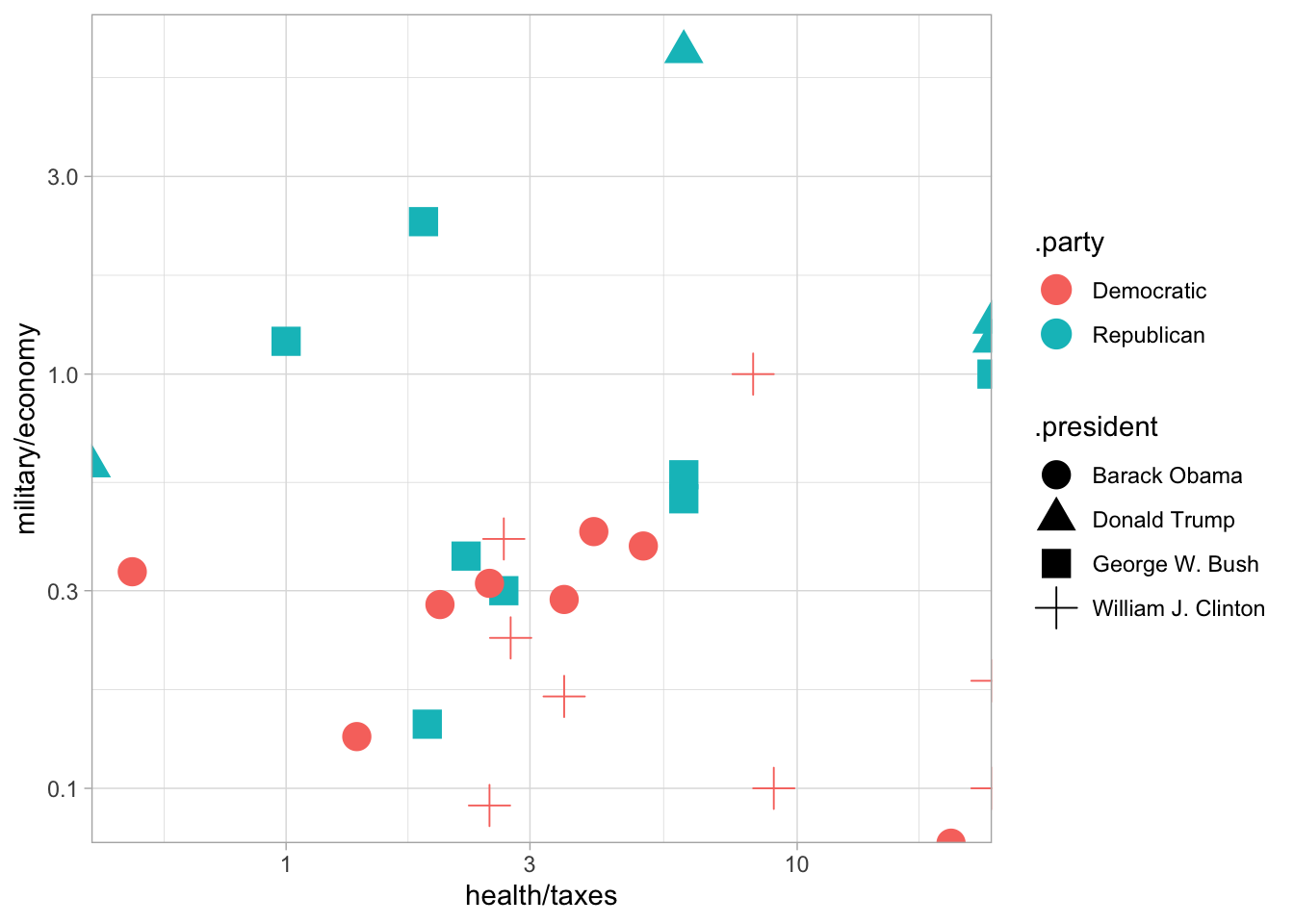
Note that we can get even more complicated: for instance, adding together lots of different words by using math in the aesthetic definition.
td_matrix %>%
  filter(.year > 1992) %>%
  ggplot() + aes(x = health / taxes, y = military / economy, color = .party, pch = .president) + geom_point(size = 5) + scale_x_log10() + scale_y_log10()
## Warning: Transformation introduced infinite values in continuous x-axis## Warning: Transformation introduced infinite values in continuous y-axis
As a challenge–can you come up with a chart that accurately distinguishes between Democrats and Republicans?
There’s a big problem with this data: it’s not normalized. Bill Clinton used to talk, a lot, in his state of the union speeches. (We can prove this with a plot)
counts %>%
  group_by(year) %>%
  summarize(count = sum(count)) %>%
  ggplot() + aes(x = as.numeric(year), y = count) + geom_line()
We can normalize these plots so that the term-document matrix gives the relative use per words of text. By setting ratio = count/sum(count) inside a mutute call, you get the percentage of the count.
normalized = counts %>%
  group_by(year) %>%
  mutate(ratio = count / sum(count)) %>%
  ungroup()


normalized %>%
  filter(word == "i") %>%
  ggplot() + aes(x = as.numeric(year), y = ratio) + geom_line() + scale_y_continuous(label = scales::percent)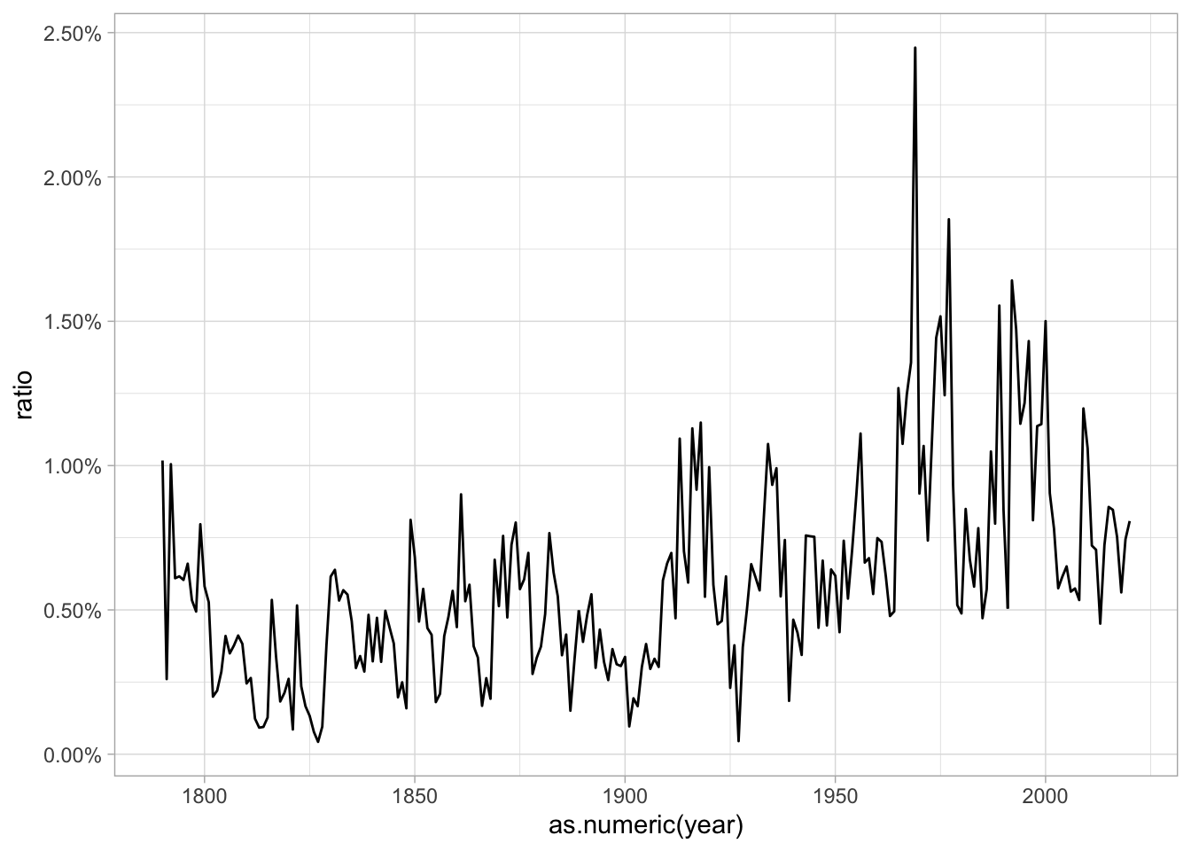
norm_data_frame = normalized %>%
  group_by(word) %>%
  filter(mean(ratio) > .0005) %>%
  select(-count)

norm_td_matrix = norm_data_frame %>%
  ungroup() %>%
  mutate(.year = year) %>%
  select(-year) %>%
  spread(word, ratio, fill = 0)
If you install the rgl library, you can look at some of these plots in 3 dimensions. This is confusing; 3d plotting is almost never a good idea. But by rotating a plot in
3-d space, you can begin to get a sense of what any of these efforts do.
10.3 Principal Components and dimensionality reduction
Principal Components are a way of finding a projection that maximizes variation. Instead of the actual dimensions, it finds the single strongest line through the high-dimensional space; and then the next; and then the next; and so forth.
principal_components_model = norm_td_matrix %>%
  select(-.year) %>%
  prcomp() # Do a principal components analysis: this is built into R.

sort(-principal_components_model$rotation[,1])
## we our i and
## -2.711870e-01 -1.595339e-01 -7.073321e-02 -6.601051e-02
## will must a are
## -5.355900e-02 -5.334852e-02 -4.973141e-02 -4.637748e-02
## america you world us
## -4.618629e-02 -4.419425e-02 -4.268881e-02 -3.934082e-02
## more new this people
## -3.914871e-02 -3.766696e-02 -3.621410e-02 -3.605556e-02
## is do can americans
## -3.265080e-02 -3.186461e-02 -3.142077e-02 -3.121777e-02
## but american years help
## -3.103994e-02 -2.923009e-02 -2.798607e-02 -2.723810e-02
## that who tonight work
## -2.662525e-02 -2.563795e-02 -2.453909e-02 -2.367167e-02
## make now know tax
## -2.233148e-02 -2.184692e-02 -2.169202e-02 -2.134336e-02
## jobs all security need
## -2.109319e-02 -2.059359e-02 -1.926443e-02 -1.920891e-02
## for budget because what
## -1.888795e-02 -1.875911e-02 -1.838907e-02 -1.827800e-02
## economy economic children they
## -1.821104e-02 -1.773126e-02 -1.733622e-02 -1.692198e-02
## one nation freedom every
## -1.646536e-02 -1.644192e-02 -1.628333e-02 -1.605788e-02
## together up health today
## -1.571828e-02 -1.558404e-02 -1.541401e-02 -1.534119e-02
## it's let federal program
## -1.512143e-02 -1.510583e-02 -1.507890e-02 -1.505633e-02
## here want get we've
## -1.443672e-02 -1.389722e-02 -1.356658e-02 -1.322021e-02
## than families million billion
## -1.318752e-02 -1.316922e-02 -1.310370e-02 -1.289363e-02
## percent future down that's
## -1.273574e-02 -1.271383e-02 -1.259529e-02 -1.242571e-02
## care programs ask better
## -1.240100e-02 -1.224500e-02 -1.217676e-02 -1.199860e-02
## we're home if just
## -1.160415e-02 -1.154786e-02 -1.150477e-02 -1.150009e-02
## working about come america's
## -1.147024e-02 -1.140241e-02 -1.137078e-02 -1.118980e-02
## out year energy peace
## -1.117743e-02 -1.101010e-02 -1.086598e-02 -1.056890e-02
## when free over job
## -1.053861e-02 -1.035184e-02 -1.034565e-02 -1.025132e-02
## first next spending cannot
## -1.024894e-02 -1.017229e-02 -1.015649e-02 -1.012140e-02
## workers like way many
## -1.008528e-02 -1.001975e-02 -9.946731e-03 -9.918531e-03
## also growth support take
## -9.659081e-03 -9.543489e-03 -9.441483e-03 -9.167678e-03
## nuclear say education cut
## -9.076225e-03 -8.972926e-03 -8.941294e-03 -8.905342e-03
## life president reform continue
## -8.608805e-03 -8.579827e-03 -8.542469e-03 -8.483737e-03
## let's forces right never
## -8.337830e-03 -8.211734e-03 -8.190580e-03 -8.129473e-03
## weapons give child my
## -7.988868e-03 -7.966077e-03 -7.959078e-03 -7.948387e-03
## high believe plan applause
## -7.867938e-03 -7.815658e-03 -7.691684e-03 -7.681208e-03
## income where challenge hope
## -7.398840e-03 -7.350181e-03 -7.349045e-03 -7.345329e-03
## defense i'm soviet time
## -7.313594e-03 -7.244082e-03 -7.219141e-03 -7.186296e-03
## don't allies so thank
## -7.186152e-03 -7.140474e-03 -7.070615e-03 -6.875170e-03
## inflation strength good too
## -6.769003e-03 -6.688979e-03 -6.675336e-03 -6.667796e-03
## meet goal needs problems
## -6.653889e-03 -6.571917e-03 -6.492624e-03 -6.425285e-03
## have again propose businesses
## -6.408425e-03 -6.275030e-03 -6.257708e-03 -6.240282e-03
## long even own ever
## -6.080475e-03 -6.009972e-03 -5.750559e-03 -5.719235e-03
## parents i've me am
## -5.709793e-03 -5.672792e-03 -5.590422e-03 -5.473022e-03
## democracy through terrorists iraq
## -5.469078e-03 -5.290707e-03 -5.061503e-03 -4.968072e-03
## can't we'll provide he
## -4.865013e-03 -4.855202e-03 -4.756954e-03 -4.649125e-03
## nations unemployment very production
## -4.624794e-03 -4.603846e-03 -4.603518e-03 -4.521473e-03
## best still medicare democratic
## -4.481724e-03 -4.475292e-03 -4.435890e-03 -4.357131e-03
## oil past they're drugs
## -4.356684e-03 -4.310702e-03 -4.099310e-03 -4.015697e-03
## use men done she
## -3.869957e-03 -3.854602e-03 -3.701944e-03 -3.693192e-03
## afghanistan there's military recovery
## -3.678904e-03 -3.677546e-03 -3.612942e-03 -3.242740e-03
## only kids business on
## -3.088624e-03 -3.066353e-03 -3.059767e-03 -2.978346e-03
## these day al progress
## -2.829985e-03 -2.776362e-03 -2.771443e-03 -2.741319e-03
## vietnam money communist national
## -2.681711e-03 -2.417290e-03 -2.375154e-03 -2.271277e-03
## terrorist iraqi there international
## -2.236987e-03 -2.219842e-03 -2.195436e-03 -2.128696e-03
## administration qaida could full
## -2.066741e-03 -1.852214e-03 -1.685798e-03 -1.585744e-03
## saddam possible before hussein
## -1.324230e-03 -1.307478e-03 -1.063447e-03 -1.024226e-03
## planes iraqis after salt
## -9.253132e-04 -8.578054e-04 -7.959238e-04 -7.630481e-04
## healthcare america’s isis iraq's
## -7.425834e-04 -7.153572e-04 -6.577789e-04 -6.399840e-04
## trade 1975 1942 already
## -6.243684e-04 -5.651995e-04 -5.613408e-04 -5.559102e-04
## some 1974 1982 sdi
## -5.523175e-04 -5.142501e-04 -5.090185e-04 -4.150049e-04
## isil rebekah axis steven
## -4.115577e-04 -3.938825e-04 -3.883216e-04 -3.841299e-04
## action 1983 system 1946
## -3.821717e-04 -3.693701e-04 -3.457709e-04 -3.447115e-04
## cory kayla barrels hitler
## -3.395937e-04 -3.384351e-04 -3.333801e-04 -3.095693e-04
## josefina ellie it’s tony
## -3.073039e-04 -2.945588e-04 -2.945588e-04 -2.921075e-04
## kenton seong increase 1947
## -2.835263e-04 -2.835263e-04 -2.759649e-04 -2.757572e-04
## sandinistas shi'a 1968 nation’s
## -2.703725e-04 -2.685607e-04 -2.526180e-04 -2.524790e-04
## each myth herman joshua
## -2.449392e-04 -2.423938e-04 -2.371998e-04 -2.371998e-04
## ashlee corey cj nazis
## -2.268210e-04 -2.268210e-04 -2.268210e-04 -2.241881e-04
## 1961 jenna megan's oliver
## -2.207340e-04 -2.173926e-04 -2.173926e-04 -2.173926e-04
## susan 250th iain janiyah
## -2.173926e-04 -2.173926e-04 -2.103992e-04 -2.103992e-04
## amy shannon afghanistan's elvin
## -2.103992e-04 -2.073860e-04 -2.073860e-04 -1.897599e-04
## alice's julie trevor 92d
## -1.897599e-04 -1.878930e-04 -1.834827e-04 -1.801126e-04
## brandon nisa's otto otto's
## -1.794703e-04 -1.701158e-04 -1.701158e-04 -1.701158e-04
## preston rebecca stacy staub
## -1.701158e-04 -1.701158e-04 -1.701158e-04 -1.701158e-04
## holets i’m i’ve jody
## -1.701158e-04 -1.683193e-04 -1.683193e-04 -1.683193e-04
## ortiz soleimani that’s hake
## -1.683193e-04 -1.683193e-04 -1.683193e-04 -1.683193e-04
## don’t kristen desiline jamiel
## -1.683193e-04 -1.667310e-04 -1.664826e-04 -1.630444e-04
## jessica megan denisha superpowers
## -1.630444e-04 -1.630444e-04 -1.630444e-04 -1.595652e-04
## judy judah schwarzkopf micheal
## -1.585141e-04 -1.423199e-04 -1.415576e-04 -1.382574e-04
## 90th safia byron 1956
## -1.379118e-04 -1.349234e-04 -1.349234e-04 -1.329126e-04
## 85th tyrone insulation forgive
## -1.240454e-04 -1.223218e-04 -1.217324e-04 -1.190166e-04
## tank goodnight wagehour beguiled
## -1.180752e-04 -1.177242e-04 -1.177242e-04 -1.177242e-04
## einstein dikembe rieman wesley
## -1.127358e-04 -1.127358e-04 -1.127358e-04 -1.127358e-04
## ingredients hats markwell prague
## -1.069528e-04 -9.284715e-05 -9.154482e-05 -9.154482e-05
## sullivan kappel debit nassau
## -9.154482e-05 -8.835034e-05 -8.549848e-05 -8.039889e-05
## 1933 hitler's fliers midway
## -7.850330e-05 -7.518450e-05 -6.963537e-05 -6.963537e-05
## reconversion eternally interrelationship 83rd
## -6.422594e-05 -6.209765e-05 -6.102518e-05 -6.075361e-05
## ostriches hull nontaxable righted
## -3.698356e-05 -1.867503e-05 -1.527633e-05 -1.448850e-05
## tapering employable underproduction abdicated
## -1.143189e-05 -1.143189e-05 8.302057e-06 1.197496e-05
## autocratic clarke huerta antagonisms
## 1.197496e-05 2.447707e-05 2.482141e-05 3.231402e-05
## excepts molestations retaliations undecaying
## 3.962125e-05 3.962125e-05 3.962125e-05 3.962125e-05
## augments lewis most interpositions
## 3.962125e-05 4.389421e-05 4.718785e-05 5.868448e-05
## involuntarily unessentially flavored visas
## 5.868448e-05 5.868448e-05 5.868448e-05 5.961042e-05
## attentions hazarded indistinctly reproached
## 6.266044e-05 6.537863e-05 6.537863e-05 6.537863e-05
## succors allured imprudence unabating
## 6.537863e-05 6.537863e-05 6.663505e-05 6.663505e-05
## unbecoming fore autocracy frankfort
## 6.663505e-05 6.663505e-05 7.438153e-05 7.601867e-05
## greytown delawares intimating licentiousness
## 7.724944e-05 8.133745e-05 8.226225e-05 8.226225e-05
## iglesias mandamus allegheny discern
## 8.388643e-05 8.405268e-05 8.489893e-05 9.334752e-05
## to enemy ungrateful deity
## 9.725961e-05 9.940147e-05 1.027430e-04 1.027430e-04
## imploring scoodiac div paredes
## 1.090845e-04 1.101644e-04 1.101644e-04 1.198361e-04
## chickamaugas violences enumerations 1857
## 1.221268e-04 1.446211e-04 1.493743e-04 2.032586e-04
## 1928 seminary toward florins
## 2.109697e-04 2.252114e-04 2.528758e-04 2.923021e-04
## well 1892 place land
## 4.187862e-04 4.810418e-04 6.546873e-04 7.251969e-04
## much yet both 1827
## 7.392304e-04 8.333437e-04 8.390984e-04 8.968164e-04
## labor since union increased
## 9.370287e-04 9.471369e-04 9.850689e-04 9.909687e-04
## legislation your against less
## 1.296139e-03 1.356695e-03 1.618757e-03 1.695436e-03
## far her 01 banks
## 1.720121e-03 1.752917e-03 1.848770e-03 1.849720e-03
## conditions those not war
## 1.892247e-03 1.956641e-03 2.065301e-03 2.268199e-03
## being course order gentlemen
## 2.287046e-03 2.450364e-03 2.583427e-03 2.697269e-03
## two no justice certain
## 2.839341e-03 2.905319e-03 3.032465e-03 3.097779e-03
## gold whether countries ought
## 3.140404e-03 3.183218e-03 3.195457e-03 3.232194e-03
## means silver policy power
## 3.301779e-03 3.360525e-03 3.387214e-03 3.447662e-03
## force militia per rights
## 3.459927e-03 3.610423e-03 3.630886e-03 3.644719e-03
## among or while fiscal
## 3.815008e-03 3.873924e-03 3.885371e-03 3.898752e-03
## cent important therefore number
## 3.980205e-03 4.000119e-03 4.086087e-03 4.134579e-03
## purpose further last given
## 4.510698e-03 4.639439e-03 4.642326e-03 4.877014e-03
## taken whole into recommend
## 4.885730e-03 4.889561e-03 4.911900e-03 4.957872e-03
## june same commission debt
## 5.173344e-03 5.201220e-03 5.209322e-03 5.554650e-03
## question army expenditures property
## 5.569736e-03 5.586378e-03 5.706589e-03 5.720734e-03
## convention them large executive
## 5.960176e-03 5.968859e-03 5.983058e-03 6.001666e-03
## governments without protection minister
## 6.109477e-03 6.152374e-03 6.209394e-03 6.213668e-03
## indians period might regard
## 6.338140e-03 6.360729e-03 6.393586e-03 6.402381e-03
## act indian authority lands
## 6.492969e-03 6.594835e-03 6.690021e-03 6.727979e-03
## measures spain country congress
## 6.869960e-03 6.877248e-03 6.950388e-03 6.980607e-03
## mexico several should provision
## 7.002003e-03 7.270598e-03 7.509774e-03 7.581245e-03
## navy commercial received having
## 7.775448e-03 7.947036e-03 8.008501e-03 8.117866e-03
## interest however british view
## 8.141896e-03 8.182902e-03 8.227947e-03 8.286503e-03
## due interests relations claims
## 8.295628e-03 8.478743e-03 8.482455e-03 8.535405e-03
## within constitution state proper
## 8.563546e-03 8.690428e-03 8.782842e-03 8.865320e-03
## effect session thus great
## 8.928975e-03 9.007666e-03 9.020563e-03 9.079339e-03
## foreign officers vessels citizens
## 9.079981e-03 9.125054e-03 9.205383e-03 9.468309e-03
## revenue duty territory part
## 9.472971e-03 9.493312e-03 9.497668e-03 9.540334e-03
## law his report powers
## 9.677301e-03 9.835395e-03 9.945818e-03 1.016905e-02
## laws secretary duties in
## 1.023864e-02 1.029327e-02 1.032166e-02 1.044580e-02
## shall amount condition service
## 1.054353e-02 1.065007e-02 1.105753e-02 1.127063e-02
## necessary department their had
## 1.132469e-02 1.173758e-02 1.175223e-02 1.303516e-02
## consideration treasury attention other
## 1.330410e-02 1.339267e-02 1.359507e-02 1.378848e-02
## commerce treaty during would
## 1.412680e-02 1.418549e-02 1.481036e-02 1.507097e-02
## any between present subject
## 1.532553e-02 1.611860e-02 1.816047e-02 1.871583e-02
## general made at were
## 1.884758e-02 1.887010e-02 1.898789e-02 1.927755e-02
## an under from public
## 1.979138e-02 2.340207e-02 2.410439e-02 2.739024e-02
## was government such as
## 3.197909e-02 3.220043e-02 3.277772e-02 3.338604e-02
## may with has its
## 3.346268e-02 3.412503e-02 3.550634e-02 3.572674e-02
## upon united it states
## 3.888852e-02 3.992784e-02 4.461992e-02 5.732890e-02
## been by be which
## 7.787905e-02 8.505783e-02 8.929235e-02 1.159745e-01
## of the
## 5.200438e-01 7.107119e-01PC_SOTUS = principal_components_model %>%
predict() %>% # Predict the pincipal components locations for each document.
as_tibble() %>% # It's an old type of data called a matrix; we want a data frame.
bind_cols(norm_td_matrix %>% select(.year)) # Attach just the years from the original which have been lost., binding along the column edges
PC_SOTUS %>% ggplot() + geom_point(aes(x = PC1, y = PC2, color = .year)) + scale_color_viridis_c()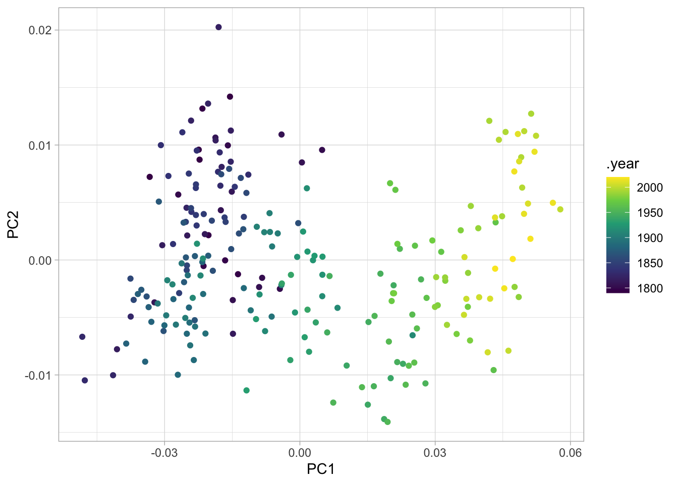
With extremely long time horizons, all separation usually happens along chronological lines. If we make the same plot, but colored by post-1980 president. Here you can see the the principal components are separating out Barack Obama and Bill Clinton separately from the other presidents.
PC_SOTUS %>%
  filter(.year > 1977) %>%
  inner_join(parties) %>%
  ggplot() +
  geom_point(aes(x = PC1, y = PC2, color = .president, pch = .party), size = 5) + scale_color_brewer(type = "qual")
## Joining, by = ".year"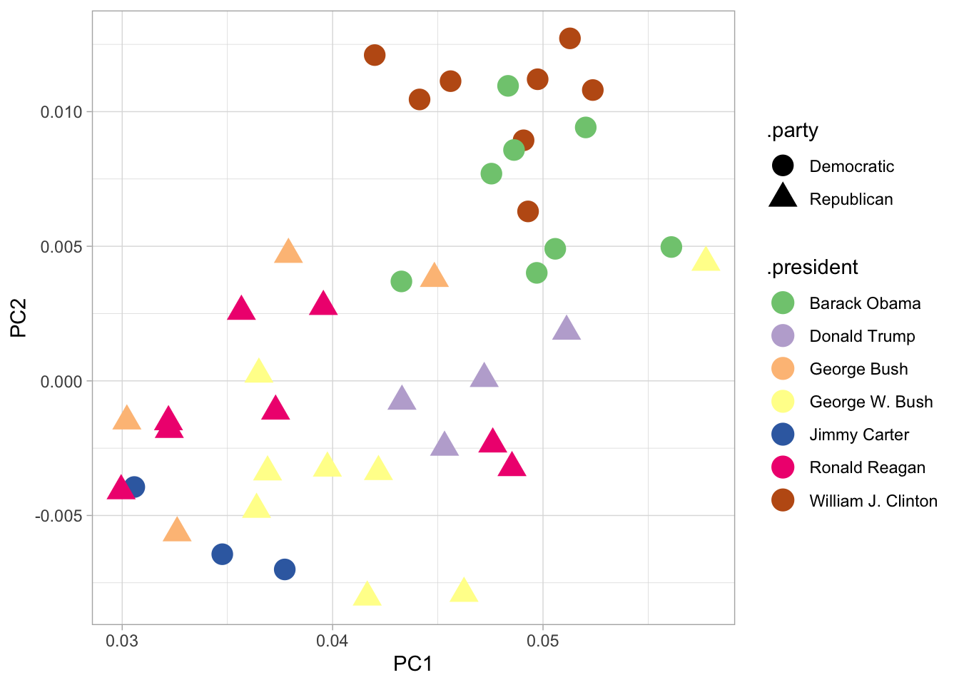
These models are created simply as weights against the word counts; we can extract those from the model by plucking the rotation element.
Definition:
pluck.pluckis a verb that works on non-data-frame element like models: it selects an element by its character name. In more traditional R,pluck(model, "rotation")might be written either asmodel[["rotation"]]or, more commonly,model$rotation.) Those methods are more concise in a line, but are awkward inside a chain.
The more modern speeches are characterized by using language like “we”, “our”, and “i”; the older ones by ‘the’, ‘of’, ‘which’, and ‘be’.
word_weights = principal_components_model %>%
  pluck("rotation") %>%
  as_tibble(rownames = "word")

word_weights %>%
  gather(dimension, weight, -word) %>%
  filter(dimension == "PC1") %>%
  arrange(-weight) %>%
  head(10)
word_weights %>%
gather(dimension, weight, -word) %>%
filter(dimension == "PC1") %>%
arrange(weight) %>%
head(10)We can plot these too! It’s a little harder to read, but these begin to cluster around different types of vocabulary.
word_weights %>%
  filter(abs(PC1) > .02) %>%
  ggplot() + geom_text(aes(x = PC1, y = PC2, label = word))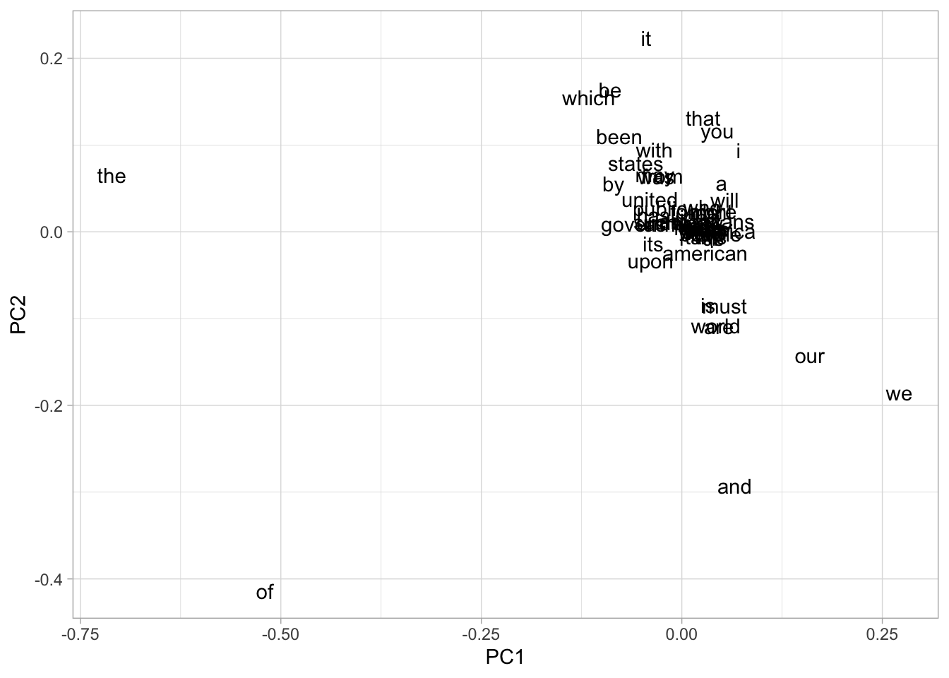
The “Word Space” that Michael describes is, in the broadest sense, related to this positioning of words together by document.@gavin_word_2018