Chapter 3 An Introduction to Data

Goals

This chapter covers the basics of types of data.

You should be able to understand what “types” of data are, and how different types of data have different conventions for working with them. As a major example, we talk about Regular Expressions, a formal language for manipulating strings; but while this skill is indispensable in practice, in theory it’s something that you can skim past if you want once you understand the situations where you might use them.

3.1 Data Types

Maybe you’ve hear this: computers store everything as binary data. Programs, numbers, text, images: in the end, all are reduced to a soup of ones and zeros. But data is not a primordial soup; in all computer languages, there are “types.” As Alex Gil once said on the Humanist mailing list, if you imagine a circle drawn on a chalk board, it can be anything–a number zero, a letter “O,” an off switch, a mouth. Before you work with symbols in a computer, you must decide which it is. The same block of data on a hard drive can mean three completely different things depending on whether you treat it as a number, a fraction, or a letter; in order to work with digital data you have to come to terms with the ontology.

In practice, this means the basics of data are these ontologies of things. The most fundamental concept is that of data types. We’ll work with many, but there are four that are so fundamental that you cannot do any work without beginning to understand them.

3.1.1 Numbers

Numbers are data. Sometimes we think of numbers as the presumptive form of data, which isn’t quite right; but they are the one that the modern computer was tuned most explicitly to create, process, and transform.

In R, a number is represented the same way we normally do in text: by typing it in digits.

Here is how you represent a number in R:

## [1] 1789

This probably seems self-evident, but in reflecting on the limitations of computers it’s worth thinking about all the ways that a computer can’t represent this number:

In English: One thousand, seven hundred and eighty-nine. Computer languages are sort of in English; they use a number of English words. But you can probably see the absurdity of typing something like this and expecting a computer to calculate with it.
In some other notation system: MDCCXXXIX. Computers are specific in that they treat Arabic numbers as real numbers.
With formatting: 1,789. Humans use formatting on data to better understand them: but a computer expects a number to be simply a set of digits bound together.

3.1.1.1 Types of Numbers

In some data analysis, there are important distinctions between different types of numbers. This is most important when it comes to fractional and irrational numbers; although you can precisely enumerate a number like ‘4,294,967,295’ in a binary system, an irrational number like ‘pi’ can only be approximated. In some languages, like python, you will need to handle important distinctions between ‘integer’ and ‘numeric’ (or ‘floating-point’) types. In R, you are generally safe using ‘numeric’ and not worrying about the difference.

3.1.2 Textual data

If numbers are the basic data for the sciences, text is the basic type for much humanities work. The fundamental unit of text is the character; a single letter at a time. Since computers store things in binary, to store a letter on a computer means turning it into a binary number.

How many letters are there? I’ll forgive you if your knee-jerk response is “26.” But even for a lightly equipped printer, the number is much higher; there are upper-case and lower-case letters, for example, and punctuation marks, and spaces, and the numbers that we used to write ‘1789.’ Each of these requires a different number (or ‘code point’) to represent it in a computer’s internal language. In all, there are 128 letters in the world, each of which a computer represents with its own binary code.

3.1.2.1 Strings

Though we set type in characters, we read in words. So while ‘character’ is the basic type, the thing that we most often want to work with is a sequence of characters all bound together. This data type is called a ‘string’ because it lines up a bunch of characters together into a line together. It’s represented in R (as in most computer languages) with quotation marks. A string can be a single word or the full works of William Shakespeare; and it’s always represented simply as characters between quotation marks.

## [1] "Just as there are rational requirements on thought, there are rational requirements on action, and altruism is one of them."

By putting together strings of 128 characters, you can represent any idea that anyone has ever or will ever write.

3.1.2.2 Character encoding

But, you might say, wait! There aren’t just English letters; there’s the “ñ” character from Spanish? What about that? Or an o with an umlaut? And the the whole Cyrillic alphabet, and Japanese Kanji characters, and full set of Chinese texts?

This a good question, and one that took the various nationally-oriented worlds of computer interaction a surprisingly long time to fix. In the first decades of computing, every language had its own set of standards, and you would always have to tell a program if you were reading in Russian, or English, or Spanish text. Around 1990, engineers in California started to work on a unified standard for text–“Unicode”–that allows all languages to be represented in the same way; rather than having just 128 letters, it gives a extensible universe with hundreds of thousands of possible characters. Egyptian hieroglyphics,

But–and this is something that every humanist must reckon with–the difference between those first 128 letters, which is known as the ASCII set, and the rest of the unicode standard remains significant. Some historical languages, like Sogdian,have only been added as of 2018; other languages are still in flux, such as the lowercase Cherokee letters added in 2015.

3.1.3 Other data types, vectors, and dataframes.

3.1.3.1 Other primitive types

Strings and characters are not the only basic data types; there are also a number of other types. Two other important ones are “logical” (which is always either TRUE or FALSE) and date.

There are also categorical types, where

3.1.4 Combined types

We’ll encounter many more specific types in this course. As time goes on, we’ll look at complicated data types like regression models or word embeddings; there are also simpler ones like dates and so-called ‘functions.’

Most of these are formed by combining together other data types in various ways. There are two especially important ways of combining data together.

3.1.4.1 Vectors

One is the vector. A vector is, simply, a sequence of data points of the same fundamental type. It is created by writing a comma-delineated list, and wrapping it in parenthesis with a c at the beginning. (That c is technically another basic data type called a ‘function’; we’ll explore it more later.)

What distinguishes a vector from just a sequence of elements (which is called, in R, a list is that each piece must be of the same type. A vector can contain strings or letters, but not both. In fact, if you try, R will quietly correct you by turning them into the same type.

c("a", "b", "c")

## [1] "a" "b" "c"

c(1, 2, 3)

## [1] 1 2 3

c(1, 2, "3")

## [1] "1" "2" "3"

3.1.4.2 Dataframes (tibbles)

Most data is about something.

If you add one more layer of abstraction in R you reach the “data frame.” This is the fundamental unit of data we’ll work with: it represents a series of vectors bound together into, as the name implies, a frame.

A dataframe resembles a more formalized version of a spreadsheet: it has columns that represent data series, and rows that represent a single observations.

Each of these columns has names that represent the type of data stored in them.

You can create a dataframe by defining each of the lists, as below. In reality, though, you will almost always read data in from elsewhere.

library(tidyverse)
tibble(city = c("Boston", "New York", "London"), population = c(600000, 8000000, 6000000))

3.2 Formal languages

To manipulate data, you need a formal language. Computers are literal beasts, and they require incredibly explicit instructions to get anything done. As with 1,789, computers tend to have only a single way to work with abstractions that human beings approach in a variety of ways. To work with data, you have to learn at least one of the computational ways of looking at this data.

There is no one, single thing called ‘computer programming’ that you can do or not do; and programming can take place outside of computer. There are, instead, a wide variety of formal languages–many of which have been developed for computers, but some of which precede them or work outside them–that can be used to describe operations on digital artifacts.

A formal language is at once incredibly expressive and incredibly limiting and frustrating. It is frustrating because it limits you; everyone wants to be able to just tell a computer what to do, and the train of errors that result from a basic command will drive you crazy. But it is, at the same time, expressive because it lets you describe almost anything you might want to describe. It also offers a firm vocabulary of operations that make it easier for you to think about doing things that might not occurr to you.

Here, for example, is a resilient formal language that describes one way of making sound:

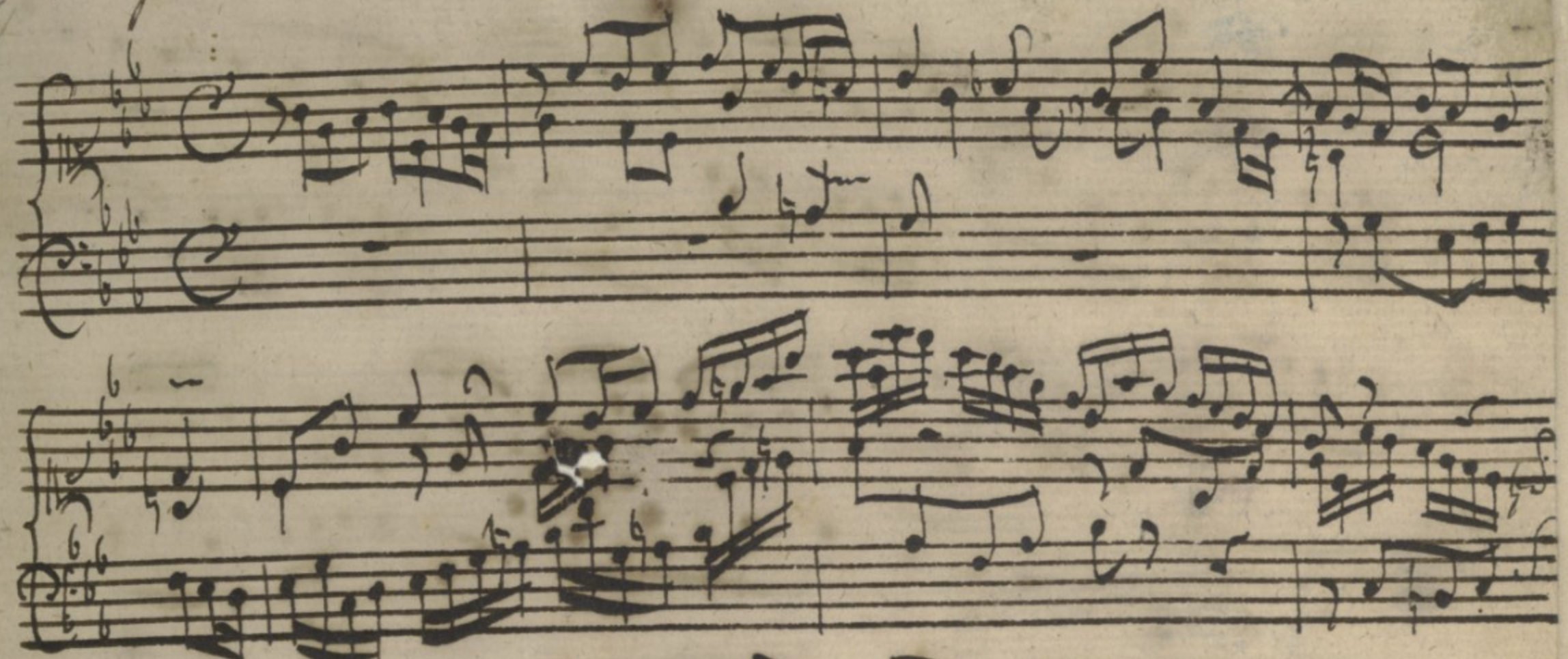Manuscript of the c-minor fugue from the Well-tempered clavier Digital Image from the British library: http://www.bl.uk/manuscripts/Viewer.aspx?ref=add_ms_35021_f001r.

Western notation builds in a number of notationary conventions that allow it concisely express music. It assumes that pitches twice as fast as each other are fundamentally the same (“octaves”), and divides the smooth spectrum of pitches between octaves into 12 ‘notes’; it encodes duration with an assumption that durations will map to the powers of two (‘quarter notes, ’eighth notes,’ ‘sixteenth notes’); and it easily encodes concurrency of multiple voices moving at the same time. Having evolved alongside a particular musical tradition, it works well at quickly allowing the assumptions of that tradition to be realized (in the piece above, Bach moves the 24 major and minor keys that had coalesced by his time); but struggles or breaks down entirely when dealing with attempts outside that tradition, as in Olivier Messiaen’s well-known attempts to transcribe birdsong in his Catalog d’oiseaux.

Messiaen, ‘Loriot’ from Catalog d’oisaeux.

This is the fundamental tension of all computer languages: that they can be expressive and generative in one dimension, but foreclose other possibilities.

Computer programmers would be lucky if they had something so expressive. A computer language is not just one thing; it usually contains a set of different strategies for working with different data types. We’ll be using ‘R’||‘Python’ in this class, but we’ll using it primarily because it’s a transparent way to execute some higher level formal languages for operating on data. One, in the packages dplyr and tidyr||module pandas, offers a way of describing things that you can do to dataframes. Another, called ggplot||altair, describes a language for describing how you build a chart out of graphical fundamentals.

One of the ways that computer languages differ from human languages is that their vocabulary is much, much more limited.

3.2.1 Arithmetic is the formal language of numbers

The most widely-used formal language for manipulating the ‘numeric type’ is incredibly complex, rule-bound, and requires a great deal of memorization. But, fortunately, you know it already as “arithmetic.”

To add up a series of fractions and then multiple them, you can write the following.

(1 / 2 + 1 / 3 + 1 / 4) * 2

## [1] 2.166667

This probably seems like commonsense. But step back to think about it for a moment. This is a notation that has little to do with the rest of R or with the internal way computers do the operations. It looks like this simply because it’s how you know to work with numbers. Some ‘purer’ languages, such as Lisp, do not bow to your middle school notation. They might force you to write out the above statement in a way the computer can process it, like (* (+ (/ 1 2) (+ (/ 1 3) (/ 1 4)) 2). But since R||Python is build to make data analysis easy, not to make you think like a computer, you can generally type arithmetic expressions in the way that you know. Parenthesis, plus and minus, and the rest are the same as in middle school.

The only major caveats to be aware of stem from the way that keyboards and the ASCII set work, i.e.:

Multiplication is an asterisk (*), not an ‘x.’
Exponentiation (‘to the power of’) can be accomplished two ways: either with a caret or two asterisks. To indicate “two squared,” for example, you can write either 2**2 or 2^2.

3.2.2 Ontologies are formal languages for specific areas

Even before it meant computer programming, “coding” in the social sciences meant classifying–taking a variety of events in the real world and turning them into data by grouping them into categories. An irreducible challenge in working with data is that it frequently demands a taxonomy, an ontology, or a controlled vocabulary. The entries in a dataset must be somehow commensurate; often this happens by applying labels to them. Animals belong to species, people belong to nationalities, books belong to genres. This can be tricky, because every classification is also an exercise in power.

Working with humanistic data requires a flexible approach to the strictness of ontologies. If you want to see the world without categories, there’s little that a computer can do for you. But you’ll also probably lose your audience’s willingness to give you the gift of data if you

3.2.3 Regexes are the formal language of strings

While you do know arithmetic–though perhaps you have not thought of it as a formal language. On the other hand, you may never have encountered a powerful formal language of strings. There is one dominant one, and it is called ‘regular expressions’ (or ‘regexes’ for short.) Just as arithmetic lets you combine, manipulate, and describe numbers, regular expressions let you characterize and edit text.³

Like arithmetic, regexes can be a bit arbitrary and capricious. As you learn them, keep in mind that they have litle to do with the rest of the language; think of this as a warmup for computational thinking, not But anyone working with text files will often find regular expressions to be very helpful. In most digital humanities projects, you’ll spend as much time cleaning data as you’ll spend actually analyzing it. Unless you want to clean data entirely by hand, you’ll want to use some basic regular expressions to parse through them.

If you’re working on a website, too, knowing your way around regular expressions can frequently save you enormous amounts of time; rather than tediously replace the same pattern over and over again, you can simply manipulate items out.

Regular expressions (or “regexes”) are, to put it generally, a vocabulary for abstractly describing text. Any reader knows that “1785-1914” is a range of dates, or that “bs145@nyu.edu” is an e-mail address. If you have a document full of date ranges, or e-mail addresses, or any other sort of text, you probably have some structured entities just like this. But a computer needs to be told what a “date range” or an “e-mail address” is. Regular expressions offer a formal language to define them, and to describe changes to them.

Regexes are more frustrating than expressive much of the time–we start with them because they’re fundamental for working with text in particular, but don’t be too put off. They require more memorization (or looking up in a table) than anything else we’ll be doing.

3.2.3.1 Examples

I used to always start off teaching regular expression by showing how powerful they are. An e-mail address, for example, can be represented with all of its portions through the following monstrosity; ^([A-Z0-9._%+-]+)@([A-Z0-9.-]+)\.([A-Z]{2,4})$. Obviously that’s longer than any single e-mail address–and I don’t expect you to read it! The point is: regular expressions let you describe strings of letters and numbers abstractly and formally. The abstraction means that you can create any sort of generalization; the formalization means that you can then use them to search, edit, or filter.

3.2.4 Where to use regexes:

If you want to unlock the full power of regular expressions, you can find them in most modern computer languages. They are even built into the Rstudio editor.

We’ll start, though, by looking at a dictionary.

It consists not just of a regular expression, but of an expression and its replacement pattern. The following little program (if you can call it that) replaces every h in a document with an i.

If you ever use the command line, the perl one-liner syntax can often be useful.

dictionary_search("worst")[1:10]

##  [1] "worst, worsted, worsting, worsts, NA, NA, NA, NA, NA, NA"
##  [2] NA                                                        
##  [3] NA                                                        
##  [4] NA                                                        
##  [5] NA                                                        
##  [6] NA                                                        
##  [7] NA                                                        
##  [8] NA                                                        
##  [9] NA                                                        
## [10] NA

3.2.5 Basic search-replace operations

3.2.5.1 Custom operators

In a regular expression, most letters mean simply themselves. If you search for Barack Obama, you’ll find the exact string “Barack Obama.”

dictionary_search("ethics")

## [1] "ethics, NA, NA, NA, NA, NA, NA, NA, NA, NA"

But a number of characters mean something different. Brackets, parentheses, and a variety of other tools have special meanings. One of the tricky things about using regexes is that you might be searching for question marks, but the question mark has its own meaning.

3.2.5.2 Basic Operators:

3.2.5.2.1 `*`, `?` and `+`

* matches the preceding character any number of times, including no times at all.
+ matches the preceding expression at least one time.
? matches the preceding expression exactly zero or one times.

3.2.5.2.2 OR: `|`

The vertical bar (sometimes called a ‘pipe’) means to search for either of two patterns. For example, if you wanted any word that has either the three letters ‘dog’ or ‘cat’ in it, you would enter the following:

dictionary_search("dog|cat")

## [1] "Alcatraz, Decatur, Hecate, Ladoga, Mercator, Muscat, Popocatepetl, Yucatan, abdicate, abdicated"

3.2.5.2.3 `.`

One last special character is the period, which matches any single character. The previous regex, for John Q. Adams, would also match “John Qz Adams,” because it has a period in it. If you’re more than forty years old or otherwised suffered through the early days of search engines, you might remember that some things had a wildcard character in them.

3.2.5.2.3.1 The power of `.*`

The most capacious regex of all is .* which tells the parser to match “any character any number of times.” There are many, many situations where this can be useful, especially combined with other regexes. A toy example is if you want to find every word that starts with a g, has a g at the end, and has a third g anywhere else.

dictionary_search("g.*g.*g")

## [1] "agglomerating, agglutinating, aggrandizing, aggravating, aggregate, aggregated, aggregates, aggregating, aggregation, aggregations"

3.2.5.3 Replacements

The syntax for replacing a regex will change from language to language, but the easiest substitution is to replace a regex by a string.

Rather than use the simple function above, we’ll use one that you’ll actually encounter in real life. Note that there are three strings in a row, separated by commas. The first is the string we’ll work on; the second is the string we want to replace; and the last is the replacement.

For instance, to replace ‘data’ with ‘capta,’ we just have to replace ‘da’ with ‘cap’:

str_replace_all("data", "da", "cap")

## [1] "capta"

3.2.6 Escape characters.

3.2.6.1 Escaping special characters

Sometimes, of course, you’ll actually want to search for a bracket, parenthesis, or other special character. To do so, you have to escape the terms. Take this, for instance:

str_replace_all("Mr. E. Science Theater", ".", "-")

## [1] "----------------------"

Since a period means ‘anything,’ this expression replaces everything in the string! That’s no good; we need a way to say ‘an actual, honest-to-god period.’ The way that we do this is with two backslashes next to each other.

(And this is one of the reasons that you have that useless backslash key on your computer; programmers use it all the time in cases like this. In most languages you need just one; in R, you need two.)

str_replace_all("Mr. E. Science Theater", "\\.", "-")

## [1] "Mr- E- Science Theater"

3.2.7 Extraction

Sometimes you want to shuffle letters around. Perhaps you want to put a name in order.

library(tidyverse)
str_extract("Bond, James", ".*,")

## [1] "Bond,"

str_extract("Bond, James", ", .*")

## [1] ", James"

str_split("Bond, James", ", ")

## [[1]]
## [1] "Bond"  "James"

3.2.7.1 Other special characters

Other important special characters come from prefacing letters.

\\n: a “newline”
\\t: a tab

(If you are working in non-English languages, there are unicode extensions that work off the special character \p (or \P to designate the inverse of a selection). \\p{L} matches any unicode letter, for example. See the unicode web site for more on this.)

3.3 Data formats

To work with data, you have to get data. But the material format of data is complicated. The types described above can vary slightly in implementation from programming language to programming language, and from computer platform to computer platform. (One change that happens at the lowest possible level of representation, which you are unlikely to ever encounter, has to do with the order of individual bits in a file; in a reference to how pointless these splits can be, computer scientists borrowed the names [“big-endian” and “little-endian”] from Gulliver’s Travels. So there need to be files that are independent of the way data is built in a computer.

The format that you receive data in will vary on the data. Text files, for example, are almost always distributed nowadays as Unicode data; books as PDFs; and images as JPGs (for small size) or TIFFs (for highest quality.)

The tabular data we’re looking at needs an on-disk format. There are few you may encounter: each has different advantages, because each serves different purposes. Economists talk about the different roles of money; it is a unit of account, a means of exchange, a store of value, etc. Data formats serve several different roles simultaneous. They can be

A permanent store for information that is likely to persist for a long time.
An interchange format that brings data between computer programs.
A means of compression. You might prefer to get images of handwritten text through your e-mail, but turning it into . In some formats, this doesn’t matter at all. Think of the way that people post photographs of books into their social media; the cost of the photograph is minimal.
An editable record that one or many people may need to collaborate on.

Different formats have different advantages. Even in the world of tabular data, there are at least four formats you are likely to encounter.

3.3.1 CSV/TSV files

The CSV format is the most basic way to share tabular data. It uses plain text to store information, so you can open it up in almost any program, but

Basically, a csv is a file in which rows are separated by return characters, and columns are separated by commas. (The TSV is an extremely similar format in which columns are instead separated by tabs; for most purposes, the two formats are interchangeable but csv sees more widespread support.)

That simple definition quickly runs into issues. What happens if a name has a comma inside of it? You can use quotes–but then what if a field has quotes inside of it? There is no single definition of a CSV. The closest is RFC 4180, which most programming languages will support; but in

CSVs can’t represent data types like null values,

3.3.2 Spreadsheets

There are two different spreadsheet programs in wide use. Microsoft Excel is a desktop program that goes back to the 1980s; Google Sheets is a web app from the 2000s. Both allow you to do a great deal of computation in them, which can mean that data gets locked into the format. They also allow a great deal of approaches that are elegant for exploring data (colored columns, merged cells) but that can make it difficult to read data into a standard form. For data entry, spreadsheets are an irreplaceable tool; if a group of people are transcribing sources together, Google Sheets can be immensely powerful. But both Excel and Google have demerits as a unit of interchange. It is possible to read directly from Google Sheets or Excel into R or Python, but often it takes some special wrangling. Their corporate ties also make them subject to decay and unsuitable as a long term archive format.

3.3.3 JSON and XML

JSON and XML are two extremely flexible text-based formats for storing data. JSON is poorly suited for tabular data, but often used anyways. Like CSVs, it is human readable, universally interpretable, and plain-text based. Unlike them, it allows for some preservation of datatypes (it can distinguish strings from integers, but not dates).

3.3.4 Apache Parquet and Apache Feather

If you want to persist data quickly, efficiently, and in a form closer to what your program works with, a new generation of binary columnar serialization formats have a number of advantages. The most widely used is Apache Parquet; another similar option is the Apache Feather format. These are formats that store columns of data contiguously as binary types, preserve datatypes rigorously, and–in the case of feather–can even support arbitrary metadata. Compared to CSV, they will take up substantially less disk space because of internal compression, and be much faster to load. If you find that you have especially large datasets, they may be worth exploring. They are not bound to any particular language. As open formats, they do not require any commercial software. But their relative youth means that they are probably not suitable for long-term storage.

The interesting thing about the feather format, in particular, is that the in-memory and on-disk representations are extremely similar. This means that feather files take much less time to load.

For both, you will need to install the Apache Arrow {{package}}.

If you wish to save intermediate work results in {{language}} nowadays, I highly recommend trying one of these instead of using CSVs or native data formats. Because they are harder to read and not so widely known, they are likely to be less suitable to sending to someone else.

3.4 Reading tabular data

Reading data into R is done using a number of functions from the readr package. In general, you should get in the habit of typing a line of code to load data and assign it to a variable. If you store your data in the same location as your code, reading a file called my_data.csv is usually as typing the following:

dataset = read_csv("my_data.csv")

Once you do this, you will have a variable called dataset storing all the columns in the file my_data.csv.

To get a more detailed walkthrough, RStudio can help you load a dataset by going to File > Import Dataset > From Text (readr). If you are doing something rather complicated like loading an Excel file, this may be useful. But for the reasons described in the first chapter, make sure that the file is still located inside the same directory (folder) as your .Rmd file or in a subfolder.

3.5 Exercises: Data and Formal Languages

3.5.1 Data Types

Two functions you’ll never use again in R are called intToUtf8 and utf8ToInt. They convert between the numbers that represent Unicode points, and the actual characters.

Vectors in R are the underlying elements of datasets. In the movie ‘2001,’ the computer is called “HAL” with the hidden joke that each of those letters are one ahead of “IBM.”

Edit this code below to take the string “Ivnbojujft” and shift its letters by one.

IBM = utf8ToInt("IBM")
intToUtf8(IBM - 1)

## [1] "HAL"

Stop and think for a second: what is the term - 1 doing above?

The numbers for I, B, and M are 73, 66, and 77 respectively. But the Unicode space is much larger. Use the intToUTf8 function to find out what character is represented by the 128,512th character in Unicode.

library(HumanitiesDataAnalysis)

Find a CSV or Excel file online and read it into R using read_csv. Assign it to a variable, and then look at what happens when the variable is printed back out. CSV reading will automatically guess at the types of data you’ve imported–does it make the right choices? Why or why not?

## 
## Attaching package: 'magrittr'

## The following object is masked from 'package:purrr':
## 
##     set_names

## The following object is masked from 'package:tidyr':
## 
##     extract

There are also formal languages for describing documents, which is a very different thing: dividing a document into sections, describing chapters, and fonts, and so forth. The most widespread in the humanities is known as TEI, which is a particular application of XML; we’ll encounter it later in this book.↩︎