Chapter 9 Working with Humanities Text Sources in R.
This chapter outlines one way of thinking about exploratory textual analysis in R.
It offers three things; the first is the most important intellectual one, while the second may offer important sources for individual people or projects.
Define a set of operations around the term-document model that avoids reifying a particular way of thinking about text–as always, already existing in “documents.” Instead, it emphasizes that that ‘document’ is a category of analysis you create, by making it represented by an operation we’ve already been using–
group_by.Giving concrete tools to do this work and other textual analysis in R on four sorts of text:
- Raw text files like the State of the Union addresses we’ve been exploring.
- “Non-consumptive” wordcount data like that distributed by JStor and the Hathi Trust that, while less rich than plain text, allows quick research at scale on an extraordinary quantity of data without much work.
- TEI and other XML-based text formats that are richer than plain text, and that have extraordinary valuable metadata about the internal structure of documents.
- (Not here, but we can talk about it more if yyou want): Bookworm, Google Ngrams, and other web services that provide aggregate count data about extremely large digital libraries.
In thinking about documents as flexible count data, to make clear that the algorithms we use for textual analysis are actually general tools of data analysis that you can use for any types of counts.
9.1 The Variable-Document model
The first principle of data analysis-as-text is what I call the ‘variable-document model.’ As we discussed last chapter, a fundamental object of many text-analysis operations is the term-document matrix, a data representation of a corpus in which
Humanities textual analysis should build off of the term-document model in exploratory work. But a major form of exploration that humanists often neglect or–worse–write off as mere pre-processing, is the act of defining a term and definining a document.
Michael Witmore wrote a wonderful article in 2010 that I routinely assign, called “The Multiple Addressibility of Text.”(witmore_multiple_2010?) The core intuition that he builds on, as a Shakespeare scholar used to dealing with a variety of manifestations of the same works, is that there are many different dimensions and scales on which text analysis proceeds. Sometimes we write about a specific line in a specific volume: sometimes we speak more generally about a much larger category like “the science fiction novel” or “incunabulae.”
The ‘book’ or the ‘document’ is best seen as just one of many different ways of looking at documents:
The book or physical instance, then, is one of many levels of address. Backing out into a larger population, we might take a genre of works to be the relevant level of address. Or we could talk about individual lines of print, all the nouns in every line, every third character in every third line. All this variation implies massive flexibility in levels of address. And more provocatively, when we create a digitized population of texts, our modes of address become more and more abstract: all concrete nouns in all the items in the collection, for example, or every item identified as a “History” by Heminges and Condell in the First Folio. Every level is a provisional unity: stable for the purposes of address but also stable because it is the object of address. Books are such provisional unities. So are all the proper names in the phone book.
9.1.1 Groupings as documents
It would be nice to have a formal language for describing the kind of operations that Witmore imagines.
In some frameworks, you do this by explicitly creating doc elements.
But in the tidyverse framework,
we have a verb that describes creating a nesting of documents this kind of process: the group_by operator.
In the functions bundled
A powerful way to treat term-document operations is thus to do any textual operations across the existing metadata groups. Suppose you want to calculate term frequencies. You can do so with the following function, that counts words:
Here’s an example of a function that does this; it’s built using the dplyr chain model (the . at the beginning is the functino argument.)
In real life, this function doesn’t generalize perfectly for two reasons
The count function assumes that you
have a token called ‘word’; but in different flows you might actually have
a bigram, or sentiment, or topic.
Additionally, it assumes that data exists as raw tidytext,
but often you will have already created a column of columns,
whether to save space or because that’s how your data is presented.
If you inspect the code to see how it looks, you’ll see the
following. There are defaults (word for the token definition,
and a series of ones for counts); and there is
dplyr’s odd quotation system for variables that uses the function enquo and the operator !!.
summarize_tf = . %>%
  count(word) %>%
  mutate(tf = n / sum(n))

sotu = read_tokens("SOTUS/2016.txt")

sotu %>%
  summarize_tf() %>%
  arrange(-tf) %>%
  filter(tf > 1 / 100) %>%
  ggplot() +
  geom_bar(aes(x = reorder(word, tf), y = tf), stat = "identity") +
  coord_flip()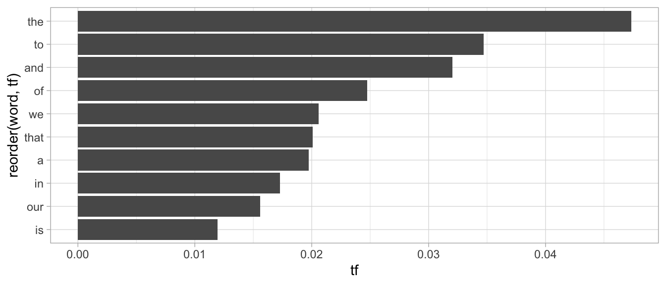
The usefulness of grouping is that you can also use it to count across multiple groups at once. If we read in two state of the unions, we can reuse almost all of this code and simply add a color parameter.
two_sotus = c("SOTUS/2016.txt", "SOTUS/2017.txt") %>%
  map_dfr(read_tokens)

two_sotus %>%
  group_by(filename) %>%
  summarize_tf() %>%
  group_by(word) %>%
  # Only terms that appear more the 1% of all words.
  filter(max(tf) > 1/100) %>%
  ggplot() +
  aes(x = reorder(word, tf), y = tf, fill = filename) +
  # (position="dodge" makes the columns appear next to each other, not stacked.)
  geom_col(position = "dodge") +
  coord_flip()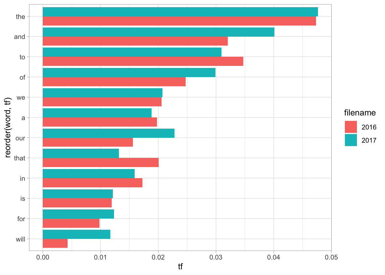
9.1.2 Chunking
Very often, it makes sense to break up a document into evenly sized chunks, which can then be used as new ‘documents.’
The add_chunks function does this for you, with a parameter ‘chunk_length.’
The chunk below divides up a State of the Union into 500-word chunks, and looks at
the most common non-stopword in each. Even this simple heuristic reveals
the path of the speech: from the economy, into sick and medical leave, to geopolitics
and finally to a discussion of civility and politics.
Don’t worry about the details of add_chunks, which uses a rather arcane set of tools in R called quosures.
Do worry about the anti_join below on stop words; it gets rids of every word
in the tidytext stop_words dataset. This builds on the
“joins as filters” strategy from the chapter on merges.
sotu %>%
  add_chunks(chunk_length = 400) %>%
  anti_join(stop_words) %>%
  group_by(chunk) %>%
  count(word) %>%
  arrange(-n) %>%
  # Take the top three words in each chunk.
  slice(1:3) %>%
  ggplot() +
  geom_text(check_overlap = TRUE) +
  aes(x = chunk, y = n, label = word)
## Joining, by = "word"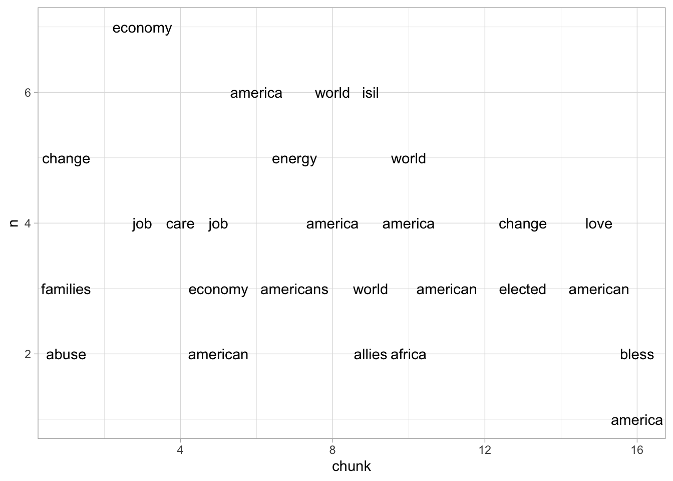
9.1.3 Programming, summarizing, and ‘binding’
Some functions like this already exist in tidytext, but the versions for this course differ in a few ways.
First, tidytext requires you to specify a document:
here, it’s created by ‘grouping.’
Second, tidytext functions are called things like bind_tf.
Here, the function is called summarize_tf,
and it performs a summarization down to a statistic for each grouping
(and word, if relevant); if you wish it to be attached to the original data, you should run a left_join operation.
9.2 TEIdytext and the variable-document model on XML
Documents come from metadata. But if you’re downloading texts yourself, you may not have that much metadata to work with.
Let’s take as an example one of the most detailed TEI transcriptions out there: the Folger library’s edition of Shakespeare’s Sonnets.
To load this in takes quite a while: currently the TEIdy function is not as quick as it could be. If someone wants to rewrite the XML parsing bits in C, I’d love to be in touch.
sonnets = TEIdy::TEIdy(system.file("extdata", "Son.xml", package = "TEIdy"))The easiest way to get a sense of what any data frame looks like is just to look at it.
This datatype can be quite difficult to look at, because TEI files have a huge amount of information in them.
As required for TEI editions, this begins with a header that contains file metadata and definitions.
The .text field contains the actual text nodes of the TEI-encoded text: the .hierarchy field tells you about the constellation of nodes that define it.
sonnets %>% head(5)If we wish to look at the actual poems, we’ll need to look at the body of the TEI element, which is required to be there. (If you’re working with non-TEI XML, there may not be a body element or a header; you can )
The Shakespeare text is remarkable in that it doesn’t require tokenization: each individual word in the document has been separately annotated in a <c> tag.
sonnets %>%
  filter(body > 0) %>%
  head(10) %>%
  select_if(~!all(is.na(.x)))
For various elements, the TEIdytext program automatically generates running counts; there are also internal counts inside the TEIdy. In general, you should always use the real TEI elements, rather than the ones created by TEIdy.
The tidy abstraction for XML works by giving column identifiers for every tag that’s present. For example, if there is a tag in
the xml like <div1 id="c1">, every text element inside it will have at least two columns with non-NA values: div1 will be an
ordered number, and div1.id will be “c1.”
Not every organizing feature exist in the TEI hierarchy. Some–like line numbers–are described through tags called `milestone``s.
This is because the organizing feature of TEI–and XML in general–is that every document must be described as a hierarchy of tags. But not all elements
don’t fit evenly into a hierarchy; a section break might fall, for instance, in the middle of the page break. milestone tags split this difference by making it possible
indicate places where breaks take.
If, for instance, we want to select every line organized by sonnet and line number, we can use tidyr::fill
to expand the milestone.n tags down.
lines = sonnets %>%
  # Make sure that there are no *other* milestones, like page numbers, in there.
  filter(is.na(milestone) || milestone.unit == "line") %>%
  # Fill in all other elements with the line number
  tidyr::fill(milestone.n) %>%
  # Select only sonnets (elements with a div2.id)
  filter(!is.na(div2.id), w > 0) %>%
  select(.text, div2.id, milestone.n)
With line numbers, now we can start to take this data in any direction, even integrating information that isn’t in the original document. For example, by creating a new dataframe that encodes the rhyme scheme and joining it against the last words, we can quickly count the most common rhymes in Shakespeare’s sonnets.
top_words = lines %>%
  group_by(.text) %>%
  summarize(count = n())

top_words %>%
  anti_join(lines %>% group_by(div2.id, milestone.n) %>% slice(n()) %>%
  ungroup() %>% select(.text)) %>%
  arrange(-count) %>% head(10)
## Joining, by = ".text"rhyme_scheme = data_frame(
milestone.n = as.character(1:14),
rhyme = c("A", "B", "A", "B", "C", "D", "C", "D", "E", "F", "E", "F", "G", "G")
)## Warning: `data_frame()` was deprecated in tibble 1.1.0.
## Please use `tibble()` instead.lines %>%
group_by(div2.id, milestone.n) %>%
slice(n()) %>% # Take the last word of each line.
inner_join(rhyme_scheme) %>% # Assign "A", "B", etc to each line.
group_by(rhyme, div2.id) %>%
arrange(.text) %>% # Arrange in alphabetical order
mutate(pair = c("first", "second")) %>%
# Drop the line number to make the spread operation work.
select(-milestone.n) %>%
spread(pair, .text) %>%
ungroup() %>%
count(first, second) %>%
filter(n > 4) %>%
ggplot() + geom_bar(aes(x = str_c(first, second, sep = "/"), y = n), stat = "identity") + coord_flip() +
labs(title = "All rhyme pairs used at least 5 times in Shakespeare's sonnets")## Joining, by = "milestone.n"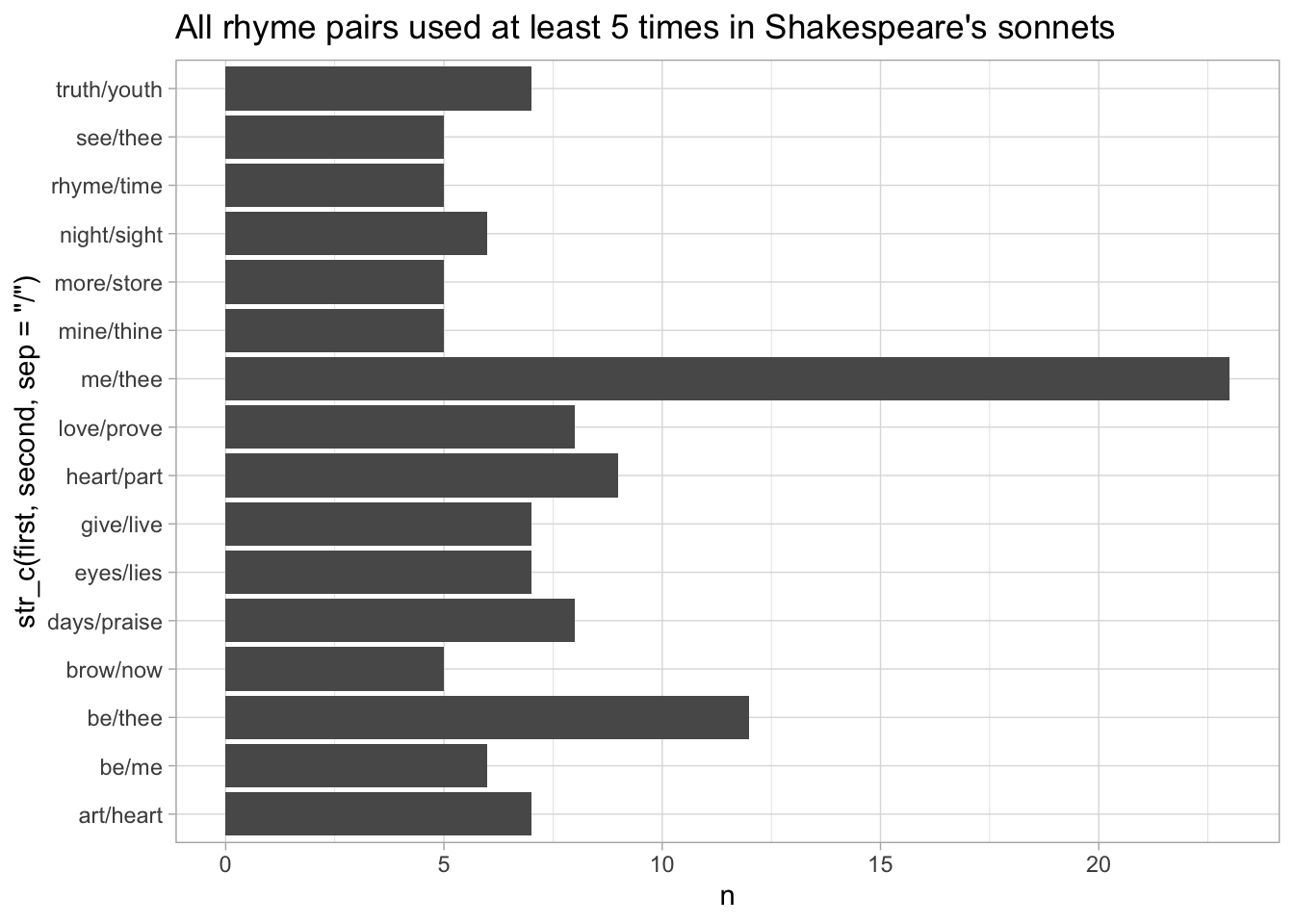
9.3 hathidy, tidyDFR, and the variable-document model for wordcounts.
A second kind of widespread text document are word counts. The Hathi Trust has made available 15 million volumes of text with word counts at the page level.13
The purpose of this package is to allow you to quickly work with tidy-formatted data for any of these books. These features are useful input into a wide variety of tasks in natural language processing, visualization, and other areas.
As an example, let’s take a 1910s set of books about the American nursing profession. There are a variety of ways to get Hathi Trust IDs, especially the “Hathifiles” distributed by them; here, I’m giving just some of them directly.
htids = c("uma.ark:/13960/t8mc9ss6h", "uma.ark:/13960/t1gj0c45p", "uma.ark:/13960/t6737n84p", "uma.ark:/13960/t2v41kv5h", "uma.ark:/13960/t47p9vg3f", "uma.ark:/13960/t10p1xn5f", "uma.ark:/13960/t2q53g85h", "uma.ark:/13960/t56d6qg69", "uma.ark:/13960/t2v41kv60", "uma.ark:/13960/t0sq9r83q", "uma.ark:/13960/t49p3x80g", "uma.ark:/13960/t7kp8w06k", "uma.ark:/13960/t0dv2df4m", "uma.ark:/13960/t9r21t815", "uma.ark:/13960/t3nw0b89j", "uma.ark:/13960/t24b3z37g", "uma.ark:/13960/t7mp5ww4f", "uma.ark:/13960/t6b28qz3z", "uma.ark:/13960/t3tt5gr59", "uma.ark:/13960/t5r796r81", "uma.ark:/13960/t6qz33n9v", "uma.ark:/13960/t4cn8017q", "uma.ark:/13960/t6zw29x15", "uma.ark:/13960/t0vq3t166", "uma.ark:/13960/t05x3659v", "uma.ark:/13960/t93787880", "uma.ark:/13960/t4fn21t7s", "uma.ark:/13960/t84j1c96m", "uma.ark:/13960/t8qc0wg3s", "uma.ark:/13960/t4rj59v9d", "uma.ark:/13960/t9x06zq79", "uma.ark:/13960/t79s2mv58", "uma.ark:/13960/t73v0fh87")With hathidy, you set a directory on your computer to hold Hathi Trust volumes that will be shared across multiple projects;
the first call will download them, and subsequent ones will simply reload from your stored files.
library(hathidy)
options(hathidy_dir = "~/feature-counts/")
nursing = hathi_counts(htids,metadata = c("htid", "enumerationChronology")) %>%
  mutate(year = enumerationChronology %>% str_extract("19..") %>% as.numeric)
Once the HTIDs are known, we can load the data in. Note the global directory at the front here. It’s off by default, again so this can live online: but I strongly recommend filling in this field whenever using the package. You can store features in the current working directory, (probably in a folder called “features”), or use a global one. If you think you might work with Hathi more than once, having a local location might make sense: but for reproducible research, you should store just the files used in this particular project. If you don’t specify any location, feature counts will be downloaded to a temporary directory and deleted at the end of the session, which is less than ideal. (Among other things, your code will take much, much longer to run on a second or third run.)
You can get an overview of just the words per page in these volumes. This instantly makes clear that the later volumes of this issue change the way that they count.
nursing %>%
  group_by(page, htid, year) %>%
  summarize(count = sum(count)) %>%
  ggplot() +
  geom_tile(aes(x = page, y = year, fill = count)) +
  scale_fill_viridis_c("Words on page") +
  labs(title = "Words per page by volume.")
## `summarise()` has grouped output by 'page', 'htid'. You can override using the `.groups` argument.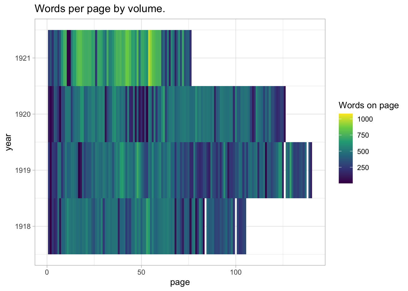
When are they talking about the ‘flu’ here? We’ll look here.
nursing %>%
  ungroup() %>%
  filter(token %>% str_detect("[Ff]lu")) %>%
  group_by(token) %>%
  # Only words that appear more than twice
  filter(sum(count) > 2) %>%
  ggplot() +
  geom_point(aes(x = year, y = token), alpha = 0.33, position = "jitter") +
  scale_color_brewer(type = "qual") +
  labs(title = "All words that use the regex '[Ff]lu'", subtitle = "'Flu' is not used in this journal, and 'influenza' is concentrated in 1918-1919")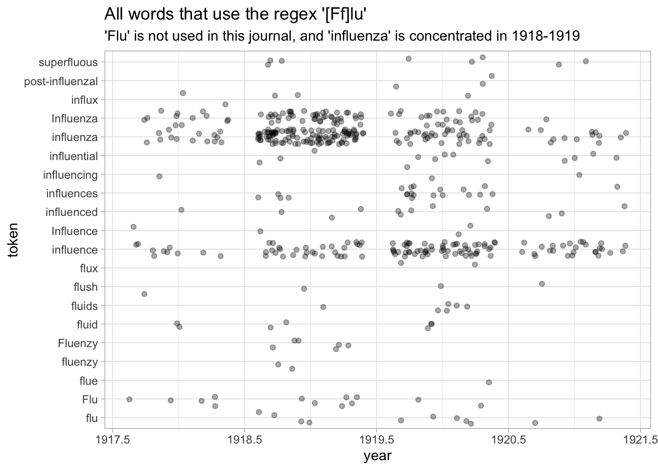
Or we can look at the usage of a word by individual issue; for this a line chart is more appropriate.
nursing %>%
  group_by(enumerationChronology) %>%
  mutate(total_words = sum(count)) %>%
  filter(token %>% tolower() == "influenza") %>%
  ggplot() + geom_col(aes(x = enumerationChronology, y = count/total_words)) +
  coord_flip() +
  labs(title = "Usage of 'Influenza' by issue")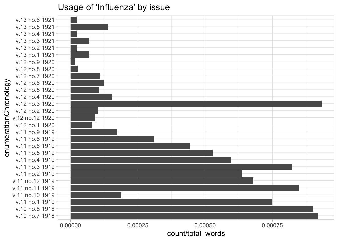
nursing %>%
  filter(token %>% tolower() == "influenza") %>%
  ggplot() + geom_point(aes(x = enumerationChronology, y = page, size = count, alpha = 0.5)) + theme_bw() +
  labs(
    title = "The 'influenza' peaks after the epidemic are clustered at individual pages."
  ) + coord_flip()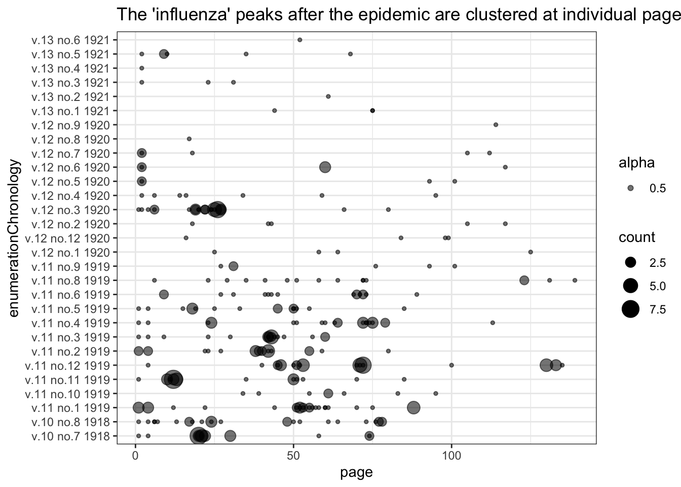
9.3.1 UNDER CONSTRUCTION
9.4 Bookworm databases
In working with Hathi, you’ll start to encounter the limits of how much data you can pull to your machine. I’ve worked with them on a project called “Bookworm” that helps you pull out information about individual words.
9.5 Exercises
9.5.1 Working with TEI
- Create a list of the 30 words that Shakespeare use most commonly, but never rhymes. (The last word of each line in a sonnet is the rhyming one.) What distinguishes them?
last_words = lines %>%
  group_by(div2.id, milestone.n) %>%
  slice(n()) %>%
  group_by(.text) %>%
  summarize(last_positions = n())

lines %>%
  count(.text) %>%
  arrange(-n) %>%
anti_join(last_words) %>% arrange(-n)- What are words that Shakespeare uses at the end of sonnets but not at the beginning?
Boris Capitanu, Ted Underwood, Peter Organisciak, Timothy Cole, Maria Janina Sarol, J. Stephen Downie (2016). The HathiTrust Research Center Extracted Feature Dataset (1.0) [Dataset]. HathiTrust Research Center,http://dx.doi.org/10.13012/J8X63JT3.↩︎