Chapter 8 Texts as Data

Research using texts is perhaps the most defining feature of digital humanities work. We’ll start by looking at one of the most canonical sets of texts out there: the State of the Union Addresses. State of the Union Addresses are a useful baseline because they are openly available and free. The files that we use here are predominantly from the American Presidency project at the University of California: https://www.presidency.ucsb.edu/documents/presidential-documents-archive-guidebook/annual-messages-congress-the-state-the-union..¹² Speeches from 2015 and later were taken straight from the White House.

library(tidyverse)
library(HumanitiesDataAnalysis)

extract_SOTUs()

We’re also going to dig a little deeper into two important aspects of R we’ve ignored so far: functions (in the sense that you can write your own) and probability.

8.1 Reading Text into R

You can read in a text the same way you would a table. But the most basic way is to take a step down the complexity ladder and read it in as a series of lines.

As a reminder, you probably need to update the package:

# devtools::install_github("HumanitiesDataAnalysis/HumanitiesDataAnalysis")

text = read_lines("SOTUS/2019.txt")

text %>% head(3)

## [1] "Madam Speaker, Mr. Vice President, Members of Congress, the First Lady of the United States, and my fellow Americans:"                                                   
## [2] "We meet tonight at a moment of unlimited potential. As we begin a new Congress, I stand here ready to work with you to achieve historic breakthroughs for all Americans."
## [3] "Millions of our fellow citizens are watching us now, gathered in this great chamber, hoping that we will govern not as two parties but as one Nation."

If you type in “text,” you’ll see that we get the full 2015 State of the Union address.

As structured here, the text is divided into paragraphs. For most of this class, we’re going to be interested instead in working with words.

8.2 Tokenization

Let’s pause and note a perplexing fact: although you probably think that you know what a word is, that conviction should grow shaky the more you think about it. “Field” and “fields” take up the same dictionary definition: is that one word or two?

In the field of corpus linguistics, the term “word” is generally dispensed with as too abstract in favor of the idea of a “token” or “type.”

Where a word is more abstract, a “type” is a concrete term used in actual language, and a “token” is the particular instance we’re interested in. The type-token distinction is used across many fields. Philosophers like Charles Saunders Pierce, who originated the term Williams (1936), use it to distinguish between abstract things (‘wizards’) and individual instances of the thing (‘Harry Potter.’) Numismatologist (scholars of coins) use it to characterize the hierarchy of coins: a single mint might produce many coins from the same mold, which is the ‘type’; each individual instance is a token of that type.

Breaking a piece of text into words is thus called “tokenization.” There are many ways to do it–coming up with creative tokenization methods will be helpful in the algorithms portion of this class. But the simplest is to simply to remove anything that isn’t a letter. Using regular expression syntax, the R function strsplit lets us do just this: split a string into pieces. We could use the regular expression [^A-Za-z] to say “split on anything that isn’t a letter between A and Z.” Note, for example, that this makes the word “Don’t” into two words.

text %>%
  str_split("[^A-Za-z]") %>%
  head(2)

## [[1]]
##  [1] "Madam"     "Speaker"   ""          "Mr"        ""          "Vice"     
##  [7] "President" ""          "Members"   "of"        "Congress"  ""         
## [13] "the"       "First"     "Lady"      "of"        "the"       "United"   
## [19] "States"    ""          "and"       "my"        "fellow"    "Americans"
## [25] ""         
## 
## [[2]]
##  [1] "We"            "meet"          "tonight"       "at"           
##  [5] "a"             "moment"        "of"            "unlimited"    
##  [9] "potential"     ""              "As"            "we"           
## [13] "begin"         "a"             "new"           "Congress"     
## [17] ""              "I"             "stand"         "here"         
## [21] "ready"         "to"            "work"          "with"         
## [25] "you"           "to"            "achieve"       "historic"     
## [29] "breakthroughs" "for"           "all"           "Americans"    
## [33] ""

You’ll notice that now each paragraph is broken off in a strange way: each paragraph shows up nested. this is because we’re now looking at data structures other than a data.frame. This can be useful: but doesn’t let us apply the rules of tidy analysis we’ve been working with. We’ve been working with tibble objects from the tidyverse. This individual word, though, can be turned into a column in a tibble by using tibble function to create it.

SOTU = tibble(text = text)

SOTU %>% head

Now we can use the “tidytext” package to start to analyze the document.

The workhorse function in tidytext is unnest_tokens. It creates a new columns (here called ‘words’) from each of the individual ones in text. This is the same, conceptually, as the splitting above,

library(tidytext)

tidied = SOTU %>%
  unnest_tokens(word, text)

You’ll notice, immediately, that this looks a little different: each of the words is lowercased, and we’ve lost all punctuation.

8.2.1 The choices of tokenization

There are, in fact, at least 7 different choices you can make in a typical tokenization process. (I’m borrowing an ontology fromo Matthew Denny and Arthur Spirling, 2017.)

1. Should words be lowercased?
2. Should punctuation be removed?
3. Should numbers be replaced by some placeholder?
4. Should words be stemmed (also called lemmatization).
5. Should bigrams or other multi-word phrase be used instead of or in addition to single word phrases?
6. Should stopwords (the most common words) be removed?
7. Should rare words be removed?

Any of these can be combined: there at least a hundred common ways to tokenize even the simplest dataset. Here are a few examples of the difference that can make, with code that shows the appropriate settings:

list(
  SOTU %>% unnest_tokens(word, text) %>% select(lowercase = word),
  SOTU %>% unnest_tokens(word, text) %>% rowwise() %>% mutate(word = SnowballC::wordStem(word)) %>% select(stemmed = word),
  SOTU %>% unnest_tokens(word, text, to_lower = F) %>% select(uppercase = word),
  SOTU %>% unnest_tokens(word, text, to_lower = F, strip_punc = FALSE) %>% select(punctuations = word),
  SOTU %>% unnest_tokens(word, text, token = "ngrams", n = 2, to_lower = F) %>% select(bigrams = word)
) %>% map_dfc(~ .x %>% head(10))

In any case, whatever definition of a word you use needs to have some use. So: What can we do with such a column put into a data.frame?

8.2.2 Wordcounts

First off, you should be able to see that the old combination of group_by, summarize, and n() allow us to create a count of words in the document.

This is perhaps the time to tell you that there is a shortcut in dplyr to do all of those at once: the count function. (A related function, add_count,

wordcounts = tidied %>%
  group_by(word) %>%
  summarize(n = n()) %>%
  arrange(-n)

wordcounts %>% head(5)

Using ggplot, we can plot the most frequent words.

8.2.2.1 Word counts and Zipf’s law.

wordcounts = wordcounts %>%
  mutate(rank = rank(-n)) %>%
  filter(n > 2, word != "")

ggplot(wordcounts) + aes(x = rank, y = n, label = word) + geom_text()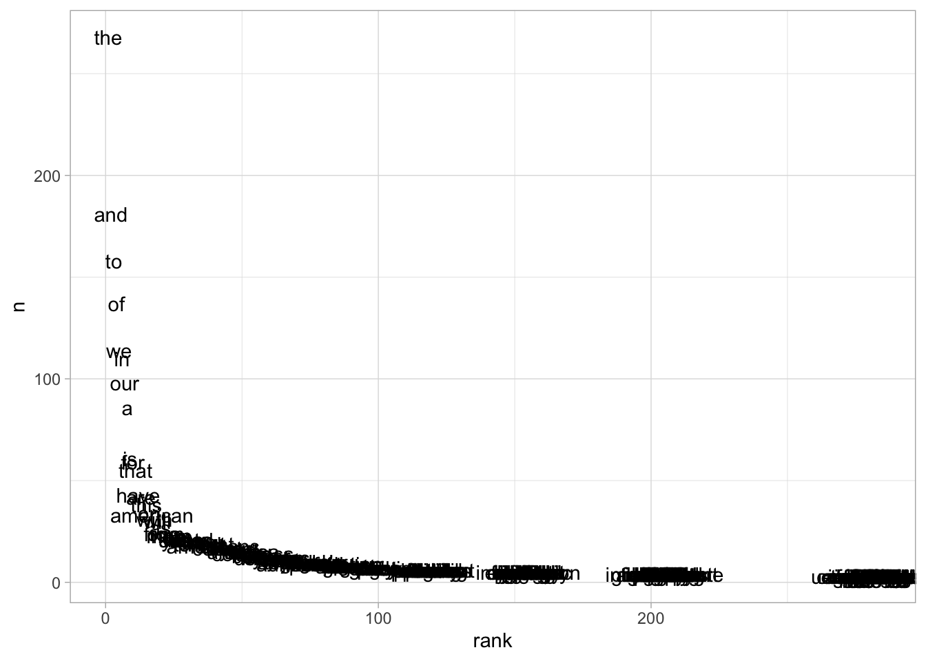

This is an odd chart: all the data is clustered in the lower right-hand quadrant, so we can barely read any but the first ten words.

As always, you should experiment with multiple scales, and especially think about logarithms.

Putting logarithmic scales on both axes reveals something interesting about the way that data is structured; this turns into a straight line.

ggplot(wordcounts) +
  aes(x = rank, y = n, label = word) +
  geom_point(alpha = .3, color = "grey") +
  geom_text(check_overlap = TRUE) +
  scale_x_continuous(trans = "log") +
  scale_y_continuous(trans = "log") +
  labs(title = "Zipf's Law",
       subtitle="The log-frequency of a term is inversely correlated with the logarithm of its rank.")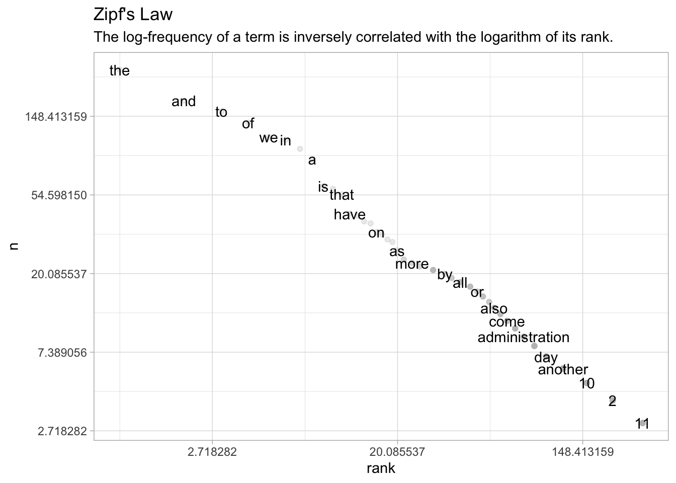

To put this formatlly, the logarithm of rank decreases linearily with the logarithm of count.

This is “Zipf’s law:” the phenomenon means that the most common word is twice as common as the second most common word, three times as common as the third most common word, four times as common as the fourth most common word, and so forth.

It is named after the linguist George Zipf, who first found the phenomenon while laboriously counting occurrences of individual words in Joyce’s Ulysses in 1935.

This is a core textual phenomenon, and one you must constantly keep in mind: common words are very common indeed, and logarithmic scales are more often appropriate for plotting than linear ones. This pattern results from many dynamic systems where the “rich get richer,” which characterizes all sorts of systems in the humanities. Consider, for one last time, our city population data.

nowadays = CESTA %>%
  arrange(-`2010`) %>% 
  mutate(rank = rank(-`2010`)) %>% 
  filter(rank < 1000)

ggplot(nowadays) + aes(x = rank, label = CityST, y = `2010`) +
  geom_point(alpha = 1, color = "grey") +
  geom_text(check_overlap = TRUE, adj = -.1) +
  scale_x_continuous(trans = "log") +
  scale_y_continuous(trans = "log")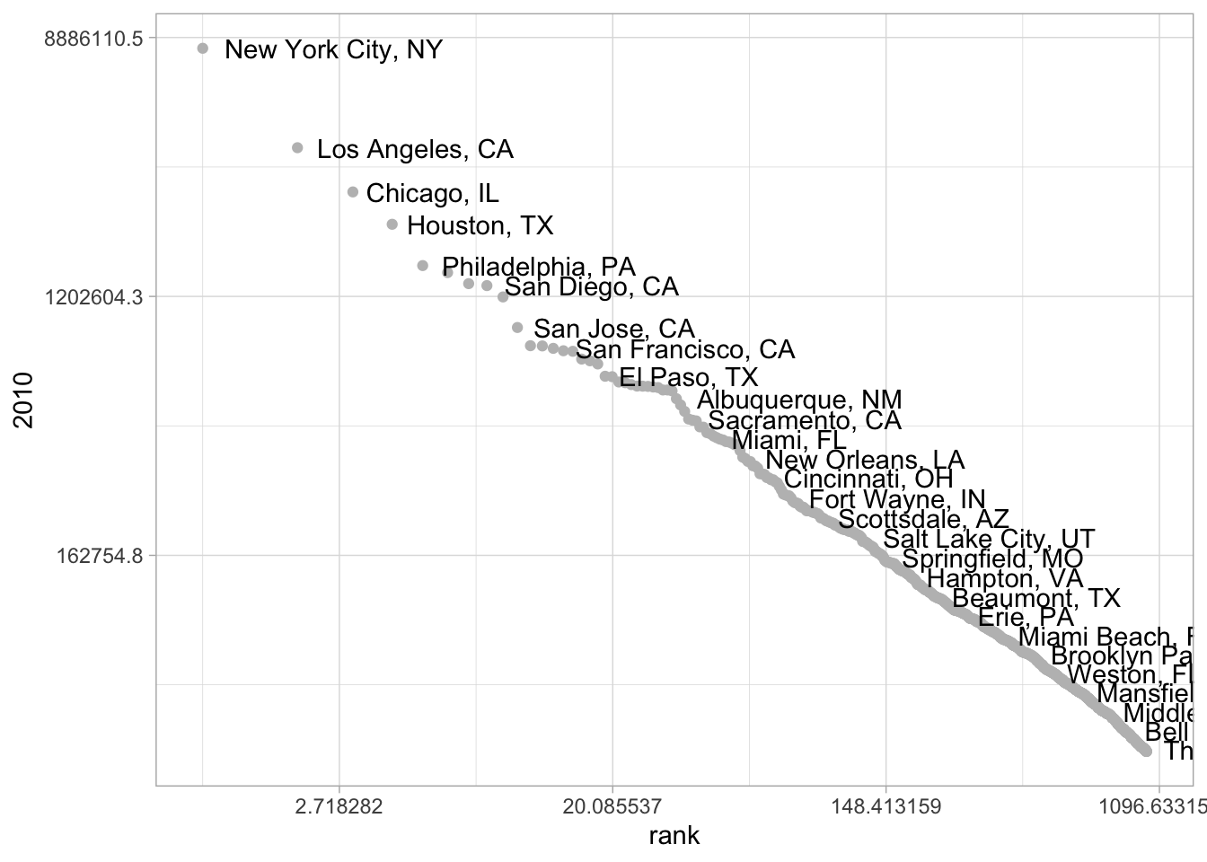

It shows the same pattern. New York is about half again as large as LA, which is a third again as large as Chicago, which is 25% as large as Houston… and so forth down the line.

(Not every country shows this pattern; for instance, both Canada and Australia have two cities of comparable size at the top of their list. A pet theory of mine is that that is a result of the legacy of British colonialism; in some functional way, London may occupy the role of “largest city” in those two countries. The states of New Jersey and Connecticut, outside New York City, also lack a single dominant city.)

8.2.3 Concordances

This tibble can also build what used to be the effort of entire scholarly careers: a “concordance” that shows the usage of each individual in context. We do this by adding a second column to the frame which is not just the first word, but the second. dplyr includes lag and lead functions that let you combine the next element. You specify by how many positions you want a vector to “lag” or “lead” another one, and the two elements are offset against each other by one.

tibble(number = c(1, 2, 3, 4, 5)) %>%
  mutate(lag = lag(number, 1)) %>%
  mutate(lead = lead(number, 1))

By using lag on a character vector, we can neatly align one series of text with the words that follow. By grouping on both words, we can use that to count bigrams:

twoColumns = tidied %>% mutate(word2 = lead(word, 1))

twoColumns %>%
  group_by(word, word2) %>%
  summarize(count = n()) %>%
  arrange(-count) %>%
  head(10)

## `summarise()` has grouped output by 'word'. You can override using the `.groups` argument.

Doing this several times gives us snippets of the text we can read across as well as down.

multiColumn = tidied %>% 
  mutate(word2 = lead(word, 1),
         word3 = lead(word, 2),
         word4 = lead(word, 3),
         word5 = lead(word, 4))


multiColumn %>% count(word, word2, word3, word4, word5) %>% arrange(-n) %>% head(5)

Using filter, we can see the context for just one particular word. This is a concordance, which lets you look at any word in context.

multiColumn %>% filter(word3 == "immigration")

8.3 Functions

That’s just one State of the Union. How are we to read them all in?

We could obviously type all the code in, one at a time. But that’s bad pogramming!

To work with this, we’re going to finally discuss a core programming concepts: functions.

We’ve used functions, continuously: but whenever you’ve written up a useful batch of code, you can bundle it into a function that you can then reuse.

Here, for example, is a function that will read the state of the union address for any year.

Note that we add one more thing to the end–a column that identifies the year.

readSOTU = function(filename) {
  
  read_lines(filename) %>%
    tibble(text = .) %>%
    filter(text != "") %>%
    ## Add a counter for the paragraph number
    mutate(paragraph = 1:n()) %>%
    unnest_tokens(word, text) %>%
    mutate(filename = filename %>%
             str_replace(".*/", "") %>%
             str_replace(".txt", "")
           )
}

readSOTU("SOTUS/1899.txt") %>% slice(16:20)

We also need to know all the names of the files! R has functions for this built in natively–you can do all sorts of file manipulation programatically, from downloading to renaming and even deleting files from your hard drive.

all_files = list.files("SOTUS", full.names = T)

Now we have a list of State of the Unions and a function to read them in. How do we automate this procedure? There are several ways.

The most traditional way, dating back to the programming languages of the 1950s, would be to write a for loop. This is OK to do, and maybe you’ll see it at some point. But it’s not the approach we take in this class.

It’s worth knowing how to recognize this kind of code if you haven’t seen it before. But we aren’t using it here. Good R programmers almost never write a for-loop; instead, they use functions that abstract up a level from working on a single item at a time.

But if you’re working in–say–python, this is almost certainly how you’d do it.

allSOTUs = tibble()

for (fname in all_files) {
  allSOTUs = rbind(allSOTUs, readSOTU(fname))
}

One of the most basic ones is called “map”: it takes as an argument a list and a function, and applies the function to each element of the list. The word “map” can mean so many things that you could write an Abbot-and-Costello routine about it. It can mean cartography, it can mean a lookup dictionary, or it can mean a process of applying a function multiple times.

The tidyverse comes with a variety of special functions for performing mapping in this last sense, including one for combining dataframes by rows called map_dfr.

allSOTUs = all_files %>%
  map_dfr(readSOTU)


allSOTUs %>%
  group_by(filename) %>%
  summarize(count = n()) %>%
  ggplot() + geom_line() + aes(x = filename %>% as.numeric(), y = count) +
  labs(title = "Number of words per State of the Union")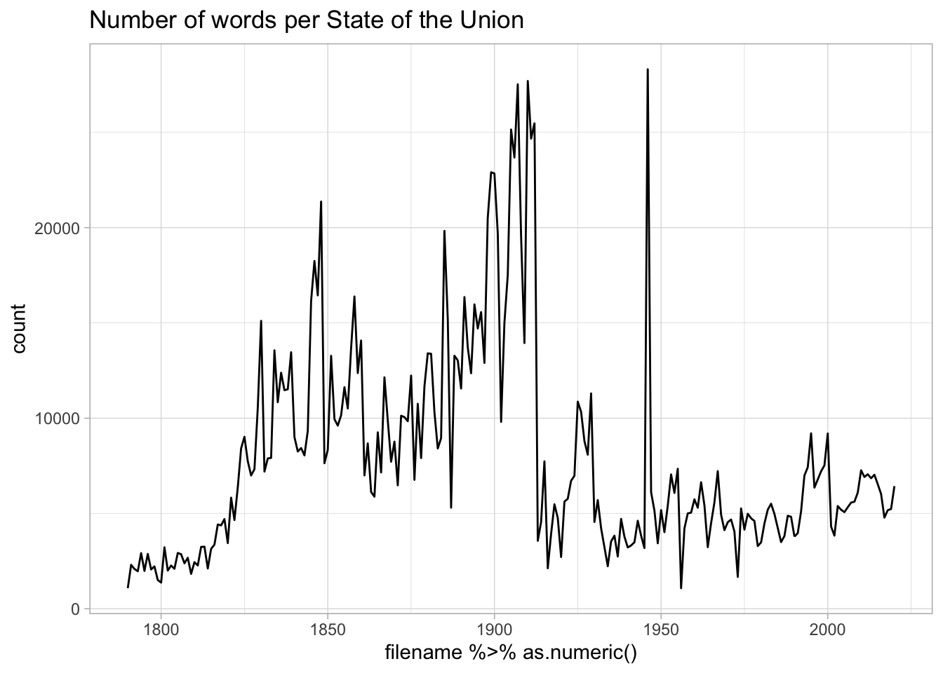

8.3.0.1 Metadata Joins

The metadata here is edited from the Programming Historian

This metadata has a field called ‘year’; we alreaday have a field called ‘filename’ that represents the same thing, except that the data type is wrong; it’s a number. So here we can fix that and do a join.

allSOTUs = allSOTUs %>%
  mutate(year = as.numeric(filename)) %>%
  inner_join(presidents)

## Joining, by = "year"

allSOTUs %>%
  ggplot() +
  geom_bar(aes(x = year, fill = party)) +
  labs("SOTU lengths by year and party")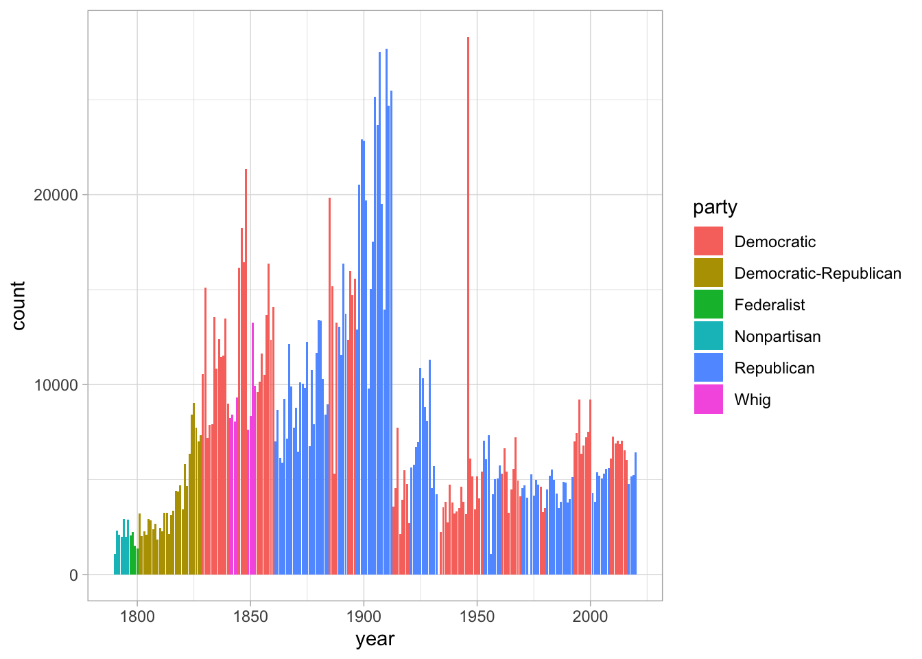

There’s an even more useful metadata field in here, though; whether the speech was written or delivered aloud.

allSOTUs %>%
  group_by(year, sotu_type) %>%
  summarize(`Word Count` = n()) %>%
  ggplot() +
  geom_point(aes(x = year, y = `Word Count`, color = sotu_type))

## `summarise()` has grouped output by 'year'. You can override using the `.groups` argument.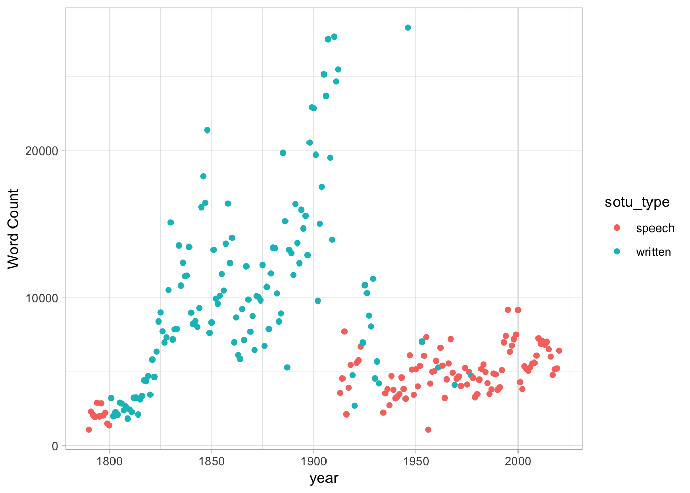

One nice application is finding words that are unique to each individual author. We can do that to find words that only appeared in a single State of the Union. We’ll put in a quick lowercase function so as not to worry about capitalization.

allSOTUs %>%
  mutate(year = as.numeric(filename)) %>%
  group_by(word, president) %>%
  summarize(count = n()) %>%
  group_by(word) %>%
  filter(n() == 1) %>%
  arrange(-count) %>% head(10)

## `summarise()` has grouped output by 'word'. You can override using the `.groups` argument.

Unique words are not the best way to make comparisons between texts: see the chapter on “advanced comparison” for a longer discussion.

8.4 Subword tokenization with sentencepiece

Some notes on integrating more complicated tokenization with tidytext in R

Tidytext works well in English, but for some languages the assumption that a “word” can be created through straightforward tokenization is more problematic. In language like Turkish or Finnish, agglutination (the composition of words through suffixes) is common; in languages like Latin or Russian, words may appear in many different forms; and in Chinese, text may not have any whitespace delineation at all.

“Sentencepiece” is one of several strategies for so-called “subword encoding” that have become popular in neural-network based natural language processing pipelines. It works by looking at the statistical properties of a set of texts to find linguistically common breakpoints.

You tell it how many individual tokens you want it to output, and it divides words up into portions. These portions may be as long as a full word or as short as a letter.

Especially common words will usually be preserved as they are. In the R implementation, sequences that start a word are prefixed with ▁: so, for instance, the most common word is “▁to” . This includes not just the word “to” but also “tough,” “tolerance,” and other things that start with “to.”

The number I give here, 4000 tokens, is fairly small. If you are doing this on a substantially sized corpus, you might want to go as high as 16,000 or more tokens. But the choice you make will undoubtedly be inflected by the language you’re working in, so above all, look at whether the segments you get seem to be occasionally useful.

if (!require(sentencepiece)) install.packages("sentencepiece")
library(sentencepiece)

8.4.1 Train a model, then tokenize

Sentencepiece doesn’t know ahead of time how it will split up words–instead, it looks at the words in your collection to determine a plan for splitting them up. This means you have an extra step–you must train your model on a list of files before actually doing the tokenization. Here, we pass it a list of all the files it should read. The model will be saved in the current directory if you want to reuse it later.

files = list.files("SOTUS", full.names = TRUE) %>% keep(~str_detect(.x, ".txt"))
model = sentencepiece(files, vocab_size = 4000 - 1, model_dir = "." )

With the model saved, you can now tokenize a list of strings with the ‘sentencepiece_encode’ function. To use the model, it needs to be passed as the first argument to the function; but we can still use the same functions to put the words in a dataframe and unnest them.

words = sentencepiece_encode(model, read_lines(files[210]))
table = data_frame(words) %>% unnest(words)

table %>% count(encoded) %>% arrange(-n)
table %>% filter(lag(encoded, 1) == "▁in") %>% count(encoded) %>% arrange(-n)

8.5 Probabilities and Markov chains.

Let’s look at probabilities, which lets us apply our merging and functional skills in a fun way.

bigrams = allSOTUs %>%
  mutate(word1 = word, word2 = lead(word, 1), word3 = lead(word, 2))

transitions = bigrams %>%
  group_by(word1) %>%
  # First, we store the count for each word.
  mutate(word1Count = n()) %>%
  group_by(word1, word2) %>%
  # Then we group1 by the second word to see what share of 
  # the first word is followed by the second.
  summarize(chance = n() / word1Count[1])

## `summarise()` has grouped output by 'word1'. You can override using the `.groups` argument.

This gives a set of probabilities. What words follow “United?”

transitions %>%
  filter(word1 == "united") %>%
  arrange(-chance) %>%
  head(5)

We can use the weight argument to sample_n. If you run this several times, you’ll see that you get different results.

transitions %>%
  filter(word1 == "my") %>%
  sample_n(1, weight = chance)

So now, consider how we combine this with joins. We can create a new column from a seed word, join it in against the transitions frame, and then use the function str_c–which pastes strings together– to create a new column holding our new text.

chain = data_frame(text = "my")

## Warning: `data_frame()` was deprecated in tibble 1.1.0.
## Please use `tibble()` instead.

chain = chain %>%
  mutate(word1 = text) %>%
  inner_join(transitions) %>%
  sample_n(1, weight = chance) %>%
  mutate(text = str_c(text, word2, sep = " "))

## Joining, by = "word1"

chain

(Are you having fun yet?) Here’s what’s interesting. This gives us a column that’s called “text”; and we can select it, and tokenize it again.

Why is that useful? Because now we can combine this join and the wordcounts to keep doing the same process! We tokenize our text; take the very last token; and do the merge.

Try running this piece of code several different times.

chain = chain %>%
  select(text) %>%
  unnest_tokens(word1, text, drop = FALSE) %>%
  tail(1) %>% inner_join(transitions) %>%
  sample_n(1, weight = chance) %>%
  mutate(text = str_c(text, word2, sep=" ")) %>%
  select(text)

## Joining, by = "word1"

chain

You can do this until your fingers get tired: but we can also wrap it up as a function. In the tidyverse, the simplest functions start with a dot.

add_a_word = . %>%
  select(text) %>%
  unnest_tokens(word1, text, drop = FALSE) %>%
  tail(1) %>% inner_join(transitions, by = "word1") %>%
  sample_n(1, weight = chance) %>%
  mutate(text = str_c(text, word2, sep=" ")) %>%
  select(text)

tibble(text = "america") %>%
  add_a_word %>% add_a_word %>% add_a_word %>%
  add_a_word %>% add_a_word %>% add_a_word %>%
  add_a_word %>% add_a_word %>% add_a_word %>%
  add_a_word %>% add_a_word %>% add_a_word %>%
  add_a_word %>% add_a_word %>% add_a_word %>% pull(text)

## [1] "america won in connection it is the field of another shows the justness it was marked"

seed = tibble(text = "start")

for (i in 1:15) {
  seed = add_a_word(seed)
}

seed %>% pull(text)

## [1] "start on the national treasury does not quit we have the federal government and their habits"

A more head-scratching way is to use a technique called “recursion.”

Snake eating itself.

Here the function calls itself if it has more than one word left to add. This would be something a programming class would dig into; here just know that functions might call themselves!

add_n_words = function(seed_frame, n_words) {
  with_one_addition = add_a_word(seed_frame)
  if (n_words==1) {
    return(with_one_addition)
  } else {
    return(add_n_words(with_one_addition, n_words - 1))
  }
}

add_n_words(tibble(text = "chile"), 10)

length_2_transitions = allSOTUs %>%
  mutate(word1 = word, word2 = lead(word, 1), word3 = lead(word, 2)) %>%
  group_by(word1, word2, word3) %>%
  summarize(chance = n()) %>% 
  ungroup

## `summarise()` has grouped output by 'word1', 'word2'. You can override using the `.groups` argument.

length_2_transitions %>% sample_n(10)

add_a_word = . %>%
  select(text) %>%
  unnest_tokens(word1, text, drop = FALSE) %>%
  tail(1) %>% inner_join(transitions, by = "word1") %>%
  sample_n(1, weight = chance) %>%
  mutate(text = str_c(text, word2, sep=" ")) %>%
  select(text)

add_a_bigram = . %>%
  unnest_tokens(word, text, drop=FALSE) %>%
  tail(2) %>% mutate(wordpos = str_c("word", 1:n())) %>%
  pivot_wider(values_from=word,names_from = wordpos) %>%
  inner_join(length_2_transitions) %>%
  sample_n(1, weight = chance) %>%
  mutate(text = str_c(text, word3, sep=" ")) %>%
  select(text)

start = tibble(text = "united states")

start = start %>% add_a_bigram

## Joining, by = c("word1", "word2")

start %>% head(10)

8.6 Exercises

Download these problems

8.6.1 State of the Union

Let’s review some visualization, filtering, and grouping functions using State of the Union Addresses. This initial block should get you started with state of the Union Addresses

library(tidyverse)
library(HumanitiesDataAnalysis)
library(tidytext)

extract_SOTUs()

# This code can be modified to work on *any* folder of text files.
allSOTUs = list.files("SOTUS", full.names = TRUE) %>%
  map_dfr(read_tokens)

# This one is state-of-the-union specific.
allSOTUs = allSOTUs %>%
  mutate(year = as.numeric(filename)) %>%
  inner_join(HumanitiesDataAnalysis::presidents)

## Joining, by = "year"

1. What is the first word of the 7th paragraph of the 1997 State of the Union Address?

2. What was the first State of the Union address to mention “China?” (Remember that you may have made all words lowercase.)

3. What context was that first use?

4. What post-1912 spoke the most words in State of the Union addresses? (Note “spoke”; the filter here gets rid of the written reports.)

allSOTUs %>% 
  filter (sotu_type == "speech") %>%
  KEEP_GOING

5. What president had the shortest average speech? (Note: this requires two group_bys.)

allSOTUs %>% 
  filter (sotu_type == "speech") %>%
  group_by(president, year) %>% 
  KEEP_GOING

6. Make a plot of the data from the previous answer.

8.6.2 Joins

7. Create a data frame with two columns: ‘total_words’ and ‘year,’ giving the words per speech by year.

totals = KEEP_GOING()

8. Create a line chart for words related to the military.

military_counts = allSOTUs %>%
  filter(word %in% c("army", "navy", "marines", "forces")) %>%
  KEEP_GOING

9. Do the same, but with a list of religious words. In a nutshell, what’s the history of uses of religious words in State of the Unions?

(Note: the words you use here matters! I still rue a generalization I helped someone make about this dataset on incomplete data. There’s one word, in particular, that will give you the wrong idea of the pre-1820 religious language if it is not included.)

8.6.3 Free Exercise

Fill a folder with text files of your own. Read them in, and plot the usage of some words by location, paragraph, or something else. Use a different foldername than “SOTUS” below: but do move it into your personal R folder.

all_my_files = list.files("SOTUS", full.names = TRUE) %>%
  map_dfr(read_tokens) %>%
  KEEP_GOING

---

12. Gerhard Peters and John T. Woolley. “The State of the Union, Background and Reference Table.” The American Presidency Project. Ed. John T. Woolley and Gerhard Peters. Santa Barbara, CA: University of California. 1999-2020. Available from the World Wide Web: https://www.presidency.ucsb.edu/node/324107/↩︎