Dunning Amok

A few points following up my two posts on corpus comparison using Dunning Log-Likelihood last month. Nur ein stueck Technik.

Ted said in the comments that he’s interested in literary diction.

I’ve actually been thinking about Dunnings lately too. I was put in mind of it by a great article a couple of months ago by Ben ZimmerZimmerman addressing the character of “literary diction” in a given period (i.e., Dunnings on a fiction corpus versus the broader corpus of works in the same period).

I’d like to incorporate a diachronic dimension to that analysis. In other words, first take a corpus of 18/19c fiction and compare it to other books published in the same period. Then, among the words that are generally overrepresented in 18/19c fiction, look for those whose degree of overrepresentation *peaks in a given period* of 10 or 20 years. Perhaps this would involve doing a kind of meta-Dunnings on the Dunnings results themselves.

I’m still thinking about this, as I come back to doing some other stuff with the Dunnings. This actually seems to me like a case where the Dunning’s wouldn’t be much good; so much of a Dunning score is about the sizes of the corpuses, so after an initial comparison to establish ‘ literary diction ’ (say), I think we’d just want to compare the percentages.

Specifically; say “mossy” appears 10 times out of a thousand in fiction in 1858, and 100 times out of ten thousand in 1868; and that the comparison set is constant at 10 out of ten thousand. That is to say, nothing’s changed except that we have more fiction. The Dunning score will be higher for 1868, but nothing about the character of literary discourse has; I’d think in this case we’d just want to know that it appears ten times more often in fiction than in the baseline.

Actually, this shouldn’t be too hard to do, so maybe I’ll just spin it up. [[Since I started this, Ted posted some interesting stuff on using Mann-Whitney scores instead of Dunning; I’m not going to engage with that here since I already started down another road, but it’s worth reading]].

It takes a lot of time using my current system to get all the books in really large genres, so as a temporary measure I’ll just take small samples of about one to ten thousand books from each category. Running Dunning Stats on PZ, my favorite proxy for fiction (although it seems to slant more towards juvenalia than serious literature, which is probably a problem for Ted), lets us generate a list of particularly fictive words.

\> sort(-comparison)\[1:49\]
        she         you         her          he         had         was        said
\-1206331.71 -1038374.23  -868169.97  -649760.38  -496750.13  -260813.56  -233680.58
        don        look          me         him         his          my          go
 -217721.48  -210904.69  -206869.61  -170743.53  -163188.28  -138647.28  -130070.66
       know          ll       could        eyes          up      little         but
 -119696.02  -110606.00  -106066.20  -102207.69   -99798.48   -97299.37   -97279.49
         ve        face        what        back        your         did         out
  -93464.54   -91830.15   -89691.31   -83970.13   -83532.50   -82152.63   -80811.68
       girl       think       would        like        down        tell        went
  -78758.80   -76680.73   -76310.96   -74294.19   -73538.03   -73109.93   -71340.36
       knew         get          Oh         got        came     thought        come
  -71009.17   -70952.46   -70407.68   -69993.36   -68648.85   -64853.88   -64777.57
       then       asked          do        want        just         why      moment
  -64645.63   -63784.73   -63739.65   -61628.73   -60729.75   -59919.42   -59455.27 

The scores are below. Keep in mind that a Dunning score of something like 15 or 20 (it varies depending on the sample size) represents statistical significance; these are off-the-charts important, even using only one out of a hundred books for the sample. A few of these are interesting; most are pretty predictable, though.Pieces of contractions, conversational words… not so interesting, necessarily. Dunning’s predilection for ultra-common words strikes again.

At some point, I made a list of stopwords; if we exclude those, the overrepresented words look like this:

\> sort(-comparison\[!(names(comparison)) %in% stopwords\])\[1:49\]
      look       eyes     little       face       girl      think       tell
\-210904.69 -102207.69  -97299.37  -91830.15  -78758.80  -76680.73  -73109.93
      went       knew        get        got      asked       want     moment
 -71340.36  -71009.17  -70952.46  -69993.36  -63784.73  -61628.73  -59455.27
      door       turn       Miss       didn      smile        saw      stood
 -58605.09  -58457.83  -58397.37  -57102.08  -56991.56  -56838.73  -56007.04
       sat       room       talk        man      cried      voice       hand
 -55573.10  -54001.07  -53350.13  -52677.01  -52467.04  -51860.90  -50961.02
     woman       felt  something      laugh        old        boy      young
 -50533.76  -50105.91  -48859.61  -48198.84  -46296.65  -44681.84  -43998.46
      told     glance      night      seems        won       wait      heard
 -42303.72  -39290.72  -38343.88  -38311.51  -38138.96  -37179.80  -36854.77
       isn     mother   suddenly       sure     wouldn       walk       Lady
 -36733.91  -36520.81  -36255.29  -34485.38  -34112.25  -33219.47  -32421.47

To take a step back–what this is revealing are generally topical words, not necessarily as evocative as the ones that Ted’s been finding for poetry (“sweet”, “thy”, “fair”,“cheek”,etc.) I think that may be largely a function of the less distinctive style used for prose fiction; not totally sure. It might also be interesting to compare not against all books, but against just narratives; histories, say.

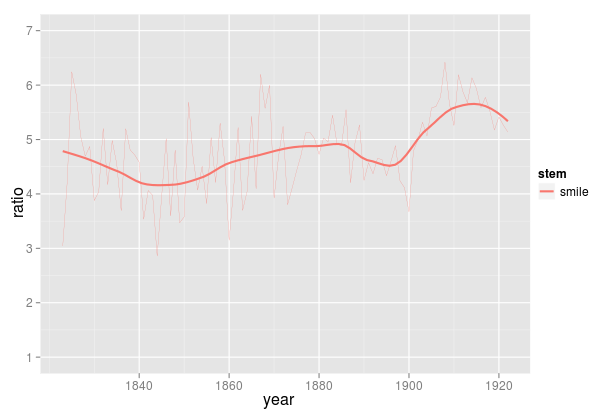
Anyhow, I think this is what we need the Dunnings for: extracting a list of words that are worth analyzing a bit more by hand. With each of these, we know there’s a real difference: we can then plot the degree of over-representation over time. I’m going to do this for the top 96 words. (Why 96? Why not?) So for instance, here’s the plot for “smile.” (Including “smiling,” “smiles,” etc.)

So “smile” drifts from being about 4x as common in fiction as in general literal literature in the 1840s up to about 5.5x by the teens.

This, it happens, is quite similar to another word in shape: “glance”

Ted’s been talking a lot about these sorts of patterns on his blog. I’ve held off much similar analysis because, mostly, of the size of my corpus. But by limiting the number of words down to about 100 using Dunning formulas to find the ones that are interesting for another reason, it then becomes more reasonable to cluster based on shape.

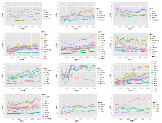
So here’s what I’m going to do. (This was developed for a slightly different project coming soon). For each of these 96 stems, I take the pattern of occurrences from 1823 to 1922: I then take the covariance matrix across that pattern, to find words that tend to move in tandem with one another. (Regardless of the absolute size of those swings.) Using kmeans clustering, I can group them into 12 (again, why not?) groups, and we can inspect the patterns for each of those groups to see what’s going on. You’ll want to click to expand this one.

There’s a lot of fairly interesting stuff going on here, although it may just be noise. Basically, we’ve got a bunch of wiggles getting classed together based on where there seem to be local peaks. (Although keep in mind that the loess regressions I use for the dark lines here are not factoring into the clustering, just the year-to-year data. So when they look strikingly similar, as in the ‘ laugh ’-‘ morning ’-‘ talk ’-‘ woman ’ cluster, that’s actually a sort of confirmation that maybe something is going right.

So, is this useful? Some of these seem pretty straightforward, such as the contractions cluster. The thing I’m most surprised by is the lack of any cluster for general downward motion; the cluster starting with “Lady” and “Miss” is some of the way there, but most words seem to become more overrepresented in fiction over time. (As I write this, I’m realizing that it’s because of a selection bias problem; I was choosing words statistically overrepresented in fiction, but since I have more books from the later 19C than the early 19C I ended up selecting for words that are particularly strong at the latter half.)

I actually think this sort of clustering/grid plot may be useful for analyzing some other phenomena, but I figured this was as good a place to any to wheel it out.

Maybe I’ll actually do a bit of reading of the clusters, and the paths they take, later. I’m curious if someone else wants to. My gut feeling here is that this needs a little bit bit more sensitivity to the groups being compared than I’m bringing here–PZ is a funny stand-in for fiction, a lot of these effects could be driven by what _else_ is in the library besides what PZ is printing, and so on.