Rejecting the gender binary: a vector-space operation
My last post provided a general introduction to the new word embedding of language (WEMs), and introduced an R package for easily performing basic operations on them. It was geared mostly towards people in the Digital Humanities community. This post looks more closely at a single word2vec model I’ve trained, on about 14 million reviews of faculty members from ratemyprofessors.com,
To be precise: it is a 500-dimensional skip-gram model with window of about 12 on lowercased, punctuation-free text using the original word2vec C code. I’ve then heavily culled the vocabulary to remove words that usually appear uppercased, on the assumption that they are proper nouns.
So just a quick refresher. My claim so far has been that WEMs offer a powerful and flexible way for thinking about relations between words in a linguistic field. Not only are words are encoded as vectors, but it is reasonable to think of the relationships between words as being meaningful themselves. The most impressive use of WEMs in the world of machine learning has been at just one sort of relationship, tasks of analogy. They are much better than any traditional methods at correctly answering SAT-style questions like “good:better::bad:???” or “fish:school::crow:???”. As I said in my last post on this, the Rate my Professor model does reasonably well on these tasks; it can, with some error, do things like correctly guess the most popular textbook in a new discipline based on previous sets of discipline-author pairs.
But insofar as WEMs work, it occurs to me that they can do much more interesting things than just solve SAT-style questions. The title of this piece is “rejecting the gender binary.” In general, that’s a phrase that tends to be used as a qualitative critical statement about cisnormativity. But WEMs actually offer us a precise formalized quantitative definition of both of these terms–“rejection” and “the gender binary”. That’s, at least, a little provocative. Of course both “gender” and “rejection” in the sense of a WEM are not the real thing: but that doesn’t mean there can’t be any possibility of insight here.
Put another way, WEMs let us take a stab formalizing an interesting counterfactual question: what would the networks of meaning in language look like if patterns that map onto gender did not exist?
  library(wordVectors)
library(dplyr)

teaching_vectors = read.vectors("~/rmp2vec/vectors.txt")
Gender as a binary
First, how do we describe gender as a binary? In the world of word2Vec, that means trying to trace out a path in space that runs from male words to female ones. Just as I was able to find a vector that the model ‘knows’ runs from disciplines to textbook authors, I can make one that runs from female to male quite easily. (The code in here is, again, using the syntax I designed for my R package.)
gender_vector = RMP[["she"]] - RMP[["he"]]
Using cosine similarity, we can extract all the words that show a heavy similarity to relational vector. Here are all the words that show a cosine similarity or dissimilarity greater than 0.25 to the gender vector. In other words, these are words that show a great deal of skew towards men or towards women.
  library(ggplot2)

word_scores = data.frame(word=rownames(RMP))
word_scores$gender_score = RMP %>% cosineSimilarity(gender_vector) %>% as.vector

ggplot(word_scores %>% filter(abs(gender_score)>.25)) + geom_bar(aes(y=gender_score,x=reorder(word,gender_score),fill=gender_score<0),stat="identity") + coord_flip()+scale_fill_discrete("Indicative of gender",labels=c("she","he")) + labs(title="The words showing the strongest skew along the gender binary")
## Warning in loop_apply(n, do.ply): Stacking not well defined when ymin != 0
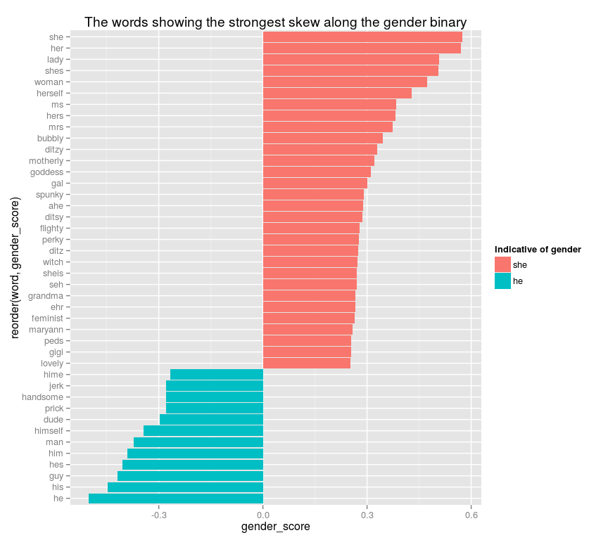
Clearly, this simple vector is capturing something significant about gendered language. We see not only a number of basic gender pronouns, but also a number of adjectives with greatly gendered application: two (“prick” and “jerk”) for male teachers, and several (“spunky”, “ditzy”, “flighty”, “feminist”,“goddess”) for women. (There are also a few names: I’ve tried to remove most of those algorithmically, but the filter didn’t catch them all.)
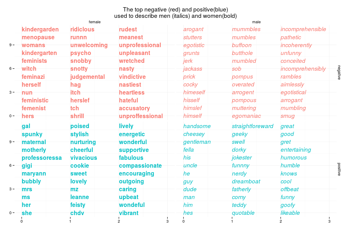
There are a lot of interesting things you can do here pull out the language of female sociology or male physical appearance. Because I want get into the rejection part pretty quickly, I’ve give just one example: a grid of the words that stick the farthest out on both of these front at once. This gives a quick sense of how students use language. (You can take any of these to my rate my professors language explorer to see a little more about how it actually breaks down.)
  goodness_vector = teaching_vectors[[c("good","best")]]-teaching_vectors[[c("bad","worst")]]

gender_vector = RMP[[c("woman","she","her","hers","ms","herself")]] - RMP[[c("man","he","his","him","mr","himself","herself")]]
word_scores$gender_score = RMP %>% cosineSimilarity(gender_vector) %>% as.vector

word_scores$goodness_score = cosineSimilarity(RMP,goodness_vector) %>% as.vector

groups = c("gender_score","goodness_score")
word_scores %>% mutate( genderedness=ifelse(gender_score>0,"female","male"),goodness=ifelse(goodness_score>0,"positive","negative")) %>% group_by(goodness,genderedness) %>% filter(rank(-(abs(gender_score*goodness_score)))<=36) %>% mutate(eval=-1+rank(abs(goodness_score)/abs(gender_score))) %>% ggplot() + geom_text(aes(x=eval %/% 12,y=eval%%12,label=word,fontface=ifelse(genderedness=="female",2,3),color=goodness),hjust=0) + facet_grid(goodness~genderedness) + theme_minimal() + scale_x_continuous("",lim=c(0,3)) + scale_y_continuous("") + labs(title="The top negative (red) and positive(blue)\nused to describe men (italics) and women(bold)") + theme(legend.position="none")
Incorporating vector rejection
So–the gender vector can extract gendered words. So far this is effectively different from other methods at generating lists of words because it is much, much faster at capturing related words for any arbitrary words.
This gets really interesting when we bring vector rejection into the picture.
Vector rejection, as I said in my last post, lets us take the take some word’s path in the word embedding and remove from all similarity to any other arbitrary vector.
So we can reject, for instance, several banking-related words from the word “bank” to get a vector that lies closest to “river.”
  chronam_vectors = read.vectors(pipe("gunzip -c ~/Dropbox/rmp2vec/shorter_chronam.txt.gz"),nrow=50000,vectors = 500)

not_that_kind_of_bank = chronam_vectors[["bank"]] %>% reject(chronam_vectors[["cashier"]]) %>% reject(chronam_vectors[["depositors"]]) %>% reject(chronam_vectors[["check"]])
chronam_vectors %>% nearest_to(not_that_kind_of_bank) %>% names
  ##  [1] "bank"     "river"    "banks"    "side"     "road"     "live"
##  [7] "lies"     "still"    "district" "tha"
This kind of straightforward rejection can be expose you to unanticipated alternate meanings of words. While looking at one of these models with some grad students, we were looking at various combinations of the vectors “colony”/“colonial”/“colonist”. I was curious at one point how the word “colony” is used in a sense independent of the word “colonist” in late 19th century newspapers. Maybe this would be India, or the Philippines. The list of words makes clear what the actual most common such context is: that of a suburb or retreat for the wealthy. (Although the presence of various island words suggests that maybe the post-1898 American empire is showing up a bit.)
chronam_vectors %>% nearest_to(chronam_vectors[["colony"]] %>% reject(chronam_vectors[["colonists"]]))
  ##    colony    suburb     group   society    island prominent  recently
## 0.3112762 0.6375631 0.6682267 0.6696360 0.6784742 0.6857096 0.6867107
##     villa   wealthy   village
## 0.6925267 0.6940062 0.6949403
Rejecting the gender binary
The distinctive feature of the new word embedding models over older matrix-based representations of language is that vectors between words have linear meaning semantically. Therefore, the process of vector rejection is meaningful on vectors between words as well as vectors of words. So here’s the formal definition of “rejecting the gender binary”; it means building a new vector space from the old by transforming each element to no longer have any directionality along the vector that separates male from female.
genderless_RMP = RMP %>% reject(RMP[["he"]]-RMP[["she"]]) %>% reject(RMP[["man"]]-RMP[["woman"]])
Compare, under these two systems, what words are closest to the word “she.” In the gendered framework, most of the words closest to “she” in meaning fall into three categories:
- obviously feminine (“her”,“lady”,“woman”,…)
- Adjectives only ever ascribed to women (“ditzy”,“bubbly”)
- Words that, like “she,” are stopwords.
RMP %>% nearest_to(RMP[["she"]],20) %>% names
  ##  [1] "she"     "her"     "shes"    "lady"    "woman"   "herself" "ms"
##  [8] "mrs"     "and"     "bubbly"  "ahe"     "that"    "very"    "it"
## [15] "also"    "hers"    "is"      "to"      "teacher" "ditzy"
In the genderless framework, the nearest words are notably different. “He” and “his” are the 2nd and fourth closing words. “Guy” is near, and “lady” and “women” fall out. General language from the corpus (“to”,“class”) replaces “ditzy” and “bubbly.” “Professor” replaces “teacher,” because students are more likely to use the more elevated title in referring to men (presumably either because women occupy more marginal instructional positions, or because students are less likely to use the more respectful title with women than with men.)
genderless_RMP %>% nearest_to(genderless_RMP[["she"]],20) %>% names
  ##  [1] "she"       "he"        "her"       "his"       "and"
##  [6] "that"      "guy"       "is"        "also"      "the"
## [11] "very"      "it"        "shes"      "to"        "s"
## [16] "really"    "but"       "class"     "professor" "you"
One nice way of expressing the differences of these two vectorspaces is to plot as a slopegraph. The left shows the most similar words and their ranks in the actual vector space, and the right shows their ranks in the vectorspace with gender removed. I show here all the words that are in the top 10 closest for either vectorspace.
slopegraph(set1="RMP",set2="genderless_RMP",word="she",10)
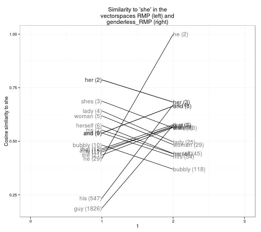
The changes are occasionally dramatic: “guy” is the 1,826th most similar word to “she” in the unadjusted space, but about the sixth closest in the adjusted one.
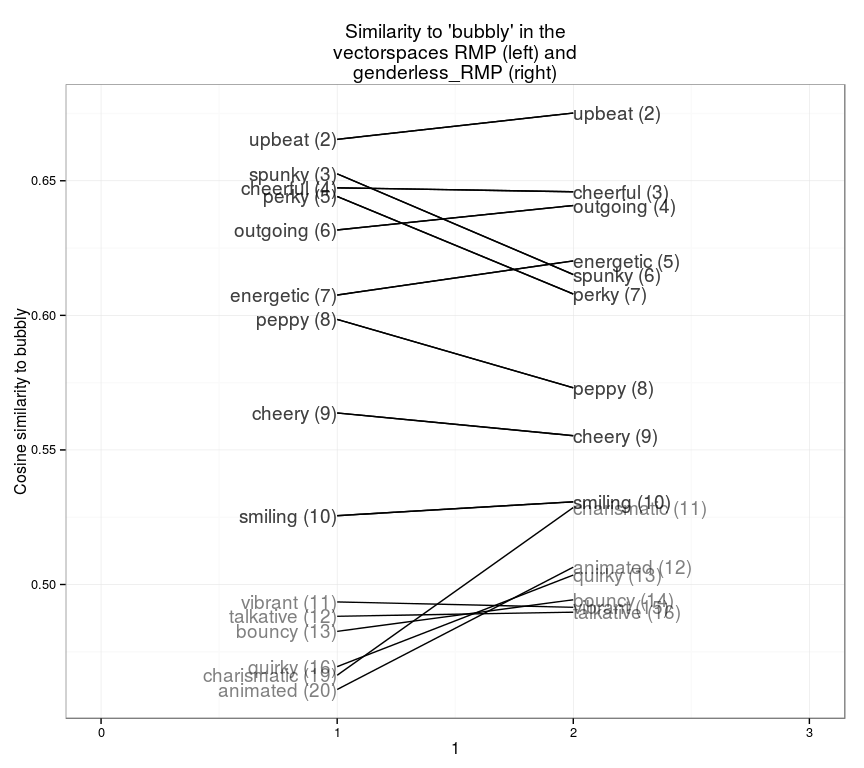
For other words, the shifts are more subtle but still noticeable. “Bubbly” has a lot of semantic meaning aside from its gender implications, so the list of words is fairly similar. But some synonyms (like “upbeat” or “energetic”) appear more similar if you factor out gender: others (like “perky” and “spunky”) seem to have been deriving a particularly large amount of their similarity from their similar gender application as opposed to other elements of context. Words that really shoot up are those like “charismatic” or “animated”, that seem to generally share a similar context with “bubbly” aside from a very different gendered application.
slopegraph(set1="RMP",set2="genderless_RMP",word="bubbly",13)
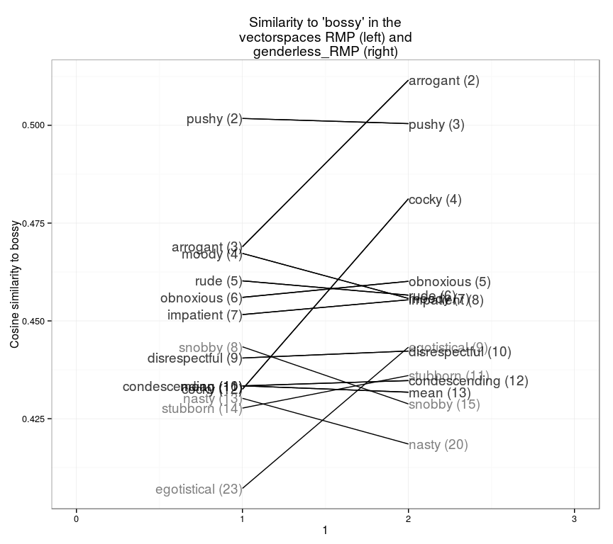
Being “bubbly” is generally a good thing: we can also explore negative words, like “bossy.” In real life, the closest word is “pushy”; but adjusting for gender, “arrogant” and “cocky” are both fairly close. (Numbering in all of these charts starts at #2: rank #1 is the word itself, which I don’t show.)
slopegraph(set1="RMP",set2="genderless_RMP",word="bossy",13)
I could just sit around exploring this space all day: in fact, I think it may be a very useful way to compare all sorts of disparate word embedding models to each other. (Eventually I’ll turn this plot at, say, 19th vs 20th century newspapers: there it could tell us how the constellation around political terms changes over time.)
But let me wrap up instead by generalizing this a little further. Let’s define a new term, “gendered synonyms.” We can say, for example, that “he” and “she” mean the same thing except that one is applied to men and the other to female. Likewise “man->woman”, “uncle->aunt”, “wife->husband”, and so forth. (Note it’s “wife->husband,” not “husband->wife”. In this language model, husbands aren’t a type of person with a gender of their own; they’re just a thing that women tend to be associated with, just like women are more likely to be associated with a “skirt” or “feminism.”)
We can generate a comprehensive list of gendered synonyms by looking for words that show a skewed gender application, and then looking for a paired word on the other side of the gender vector. Computationally, this is easily accomplished by cross comparing all the different words from the male set and the female set in the genderless space. That’s what the code below does: you can ignore it unless you’re planning to try this at home.
  ungenderize = function(model,reference) {
  model %>% reject(reference[["he"]]-reference[["she"]]) %>% reject(reference[["man"]]-reference[["woman"]])
}

masculine_RMP = RMP %>% filter_to_rownames(word_scores$word[word_scores$gender_score>.05])
feminine_RMP = RMP %>% filter_to_rownames(word_scores$word[word_scores$gender_score<(-.05)])

similarities = cosineSimilarity(feminine_RMP,masculine_RMP)
genderless_similarities = cosineSimilarity(ungenderize(feminine_RMP,RMP),masculine_RMP %>% ungenderize(RMP))

pairings = data.frame(source=rep(rownames(similarities),ncol(similarities)),target=rep(colnames(similarities),each=nrow(similarities)),true_similarity=as.vector(similarities),genderless_similarity=as.vector(genderless_similarities))

pairings = pairings %>%
  group_by(source) %>%
  mutate(source_rank=rank(-genderless_similarity)) %>%
  group_by(target) %>%
  mutate(target_rank=rank(-genderless_similarity)) %>%
  mutate(share=((1-genderless_similarity)/(1-true_similarity))) %>%
  mutate(label = paste(source,target,sep="->")) %>%
  # We don't need *everything*, and this saves memory.
  # But skip the filter for thoroughness.
  filter(source_rank<=100,target_rank<=100) %>%
  ungroup
So: we can use this to create a list of gendered synonym pairs, ordered by goodness of fit. We can call fits perfect when each word is the others closest partner in the genderless space: there are 377 word-pairs in that list. Here are the first 100, ordered by percentage of the difference between the two words that is explained by the gender vector.
At least, that’s what I’m trying to accomplish with the expression (1-genderless_similarity)/(1-true_similarity)). But I haven’t really thought through if that’s exactly the right way to compare two angles measured in radians to each other: if you know trig and want to yell at me for my transgressions, please do; I’ll listen.
  pairings %>%
    filter(source_rank<=1,target_rank<=1) %>%
    arrange(share) %>%
    head(100) %>% mutate(joint = paste(source,target,sep="->")) %>% `$`(joint)
  ##   [1] "he->she"                       "hes->shes"
##   [3] "himself->herself"              "his->her"
##   [5] "man->woman"                    "guy->lady"
##   [7] "grandpa->grandma"              "dude->chick"
##   [9] "wife->husband"                 "grandfather->grandmother"
##  [11] "dad->mom"                      "uncle->aunt"
##  [13] "fatherly->motherly"            "brother->sister"
##  [15] "actor->actress"                "grandfatherly->grandmotherly"
##  [17] "father->mother"                "genius->goddess"
##  [19] "arrogant->snobby"              "priest->nun"
##  [21] "dork->ditz"                    "handsome->gorgeous"
##  [23] "atheist->feminist"             "himmmm->herrrr"
##  [25] "kermit->degeneres"             "mans->womans"
##  [27] "hez->shez"                     "himmm->herrr"
##  [29] "trumpet->flute"                "checkride->clinicals"
##  [31] "gay->lesbian"                  "surgeon->nurse"
##  [33] "daddy->mommy"                  "cool->sweet"
##  [35] "monsieur->mme"                 "jolly->cheerful"
##  [37] "jazz->dance"                   "wears->outfits"
##  [39] "girlfriends->boyfriends"       "drle->gentille"
##  [41] "gentleman->gem"                "charisma->spunk"
##  [43] "egotistical->hypocritical"     "cutie->babe"
##  [45] "wingers->feminists"            "professore->molto"
##  [47] "gruff->stern"                  "demonstrations->activities"
##  [49] "goofy->wacky"                  "coolest->sweetest"
##  [51] "architect->interior"           "sidetracked->frazzled"
##  [53] "likeable->pleasant"            "grumpy->crabby"
##  [55] "charismatic->energetic"        "cisco->cna"
##  [57] "masculinity->gender"           "girlfriend->boyfriend"
##  [59] "king->queen"                   "sesame->kindergarden"
##  [61] "russir->cela"                  "cologne->perfume"
##  [63] "racquetball->volleyball"       "humble->compassionate"
##  [65] "simpsons->oprah"               "entertaining->lively"
##  [67] "cracking->smiling"             "chords->melody"
##  [69] "frat->sorority"                "comic->childrens"
##  [71] "philosophy->sociology"         "dj->cher"
##  [73] "chemists->nurses"              "geek->lover"
##  [75] "solidworks->indesign"          "haircut->makeover"
##  [77] "drumming->dancing"             "stagecraft->costume"
##  [79] "disgusting->nasty"             "bear->kitten"
##  [81] "sales->retail"                 "maestro->excelente"
##  [83] "quietly->kindergartners"       "willy->np"
##  [85] "mets->perso"                   "weightlifting->workout"
##  [87] "stroke->breast"                "girls->girl"
##  [89] "policing->victimology"         "evan->nonverbal"
##  [91] "biomechanics->knes"            "moe->dee"
##  [93] "absentminded->scatterbrained"  "discoveries->nutritional"
##  [95] "philosopher->sociologist"      "fungi->microbes"
##  [97] "inappropriate->unprofessional" "broadcasting->communications"
##  [99] "heap->piles"                   "hieroglyphics->rosetta"
This starts out with the most obviously gendered pronoun pairs, but quickly enters into something more interesting. Women are “nasty” while men are “disgusting.” Adorable women are “kittens”, adorable men are “[teddy] bears”
The implications of this are clearest in places where we know how to read the differences. “Goddess” may be intended as complementarily by students as is “genius,” but most academics are going to benefit more in their reviews from being called the latter. Likewise “sweet->cool”, or perhaps “activities->demonstrations.”
And there are vaguely negative words masculine words (“gruff”,“grumpy”) that years of Walter Matthau and Bill Murray movies have conditioned us to believe conceals a heart of gold: the feminine counterparts of “crabby” and “stern” feel less likely (to my ear, at least) to be redeemed.
I hope I’m succeeding at reporting stereotypes and not perpetuating them here. I know that there are parts of this whole activity that are likely to be unpalatable to some people. If you know theory and want to yell at me for my transgressions, please do; I’ll listen.
Perhaps the most interesting for me are similarities that simply reveal some of the strange ways that gender cuts across our contemporary American and Canadian college culture. Male “liberals” are “feminists”; “gender” itself is the female counterpart of “masculinity”; women teach “children’s [literature]” while men teach “comic [books].” When women do philosophy, it is called “sociology.” Mean teach policing, women teach victomology.
Just as a search bed, this promises some interesting ways to search out terms that may be sexist in ways not immediately imagined. I think there are probably some interesting applications in this sphere of automatic writing production; I can imagine a genderless autocorrect, or a bias detector, or an Orwellian series of children’s books in which adjectives are shuffled around algorithmically to de-genderize language for the next generation by making Hermione a “geek” and Hagrid “crabby” and Harry “compassionate.”
Unpaired words words
Playing along the binary in this way suggests to a certain degree that gender differences are a zero-sum-game. So it’s worth exploring as well the ways that certain words don’t have a counterpart across the aisle.
I don’t have a perfect way to do that, but one way is to say: let’s take feminine-gendered words, and then find the ones that gender does almost nothing to explain. The most extreme example of this in the set is: “thang” is gendered female. (I don’t even know what to say about that: it’s a very rare word, though.) If we ask for the closest word in the ungendered space, it is “da”; but adjusting on the ungendered axis actually increases the difference between the two words. So ungendering does very little to explain the specific meaning here.
This operation isn’t the exact opposite of the one above; in fact, a word could appear in both lists here!
  pairings %>%
    filter(source_rank==1) %>%
    mutate(percent_explained_by_shift=round(100*(genderless_similarity-true_similarity)/(1-true_similarity),5)) %>%
    select(source,target,percent_explained_by_shift,true_similarity) %>%
    arrange(percent_explained_by_shift) %>% head(20) %>% as.tbl
  ## Source: local data frame [20 x 4]
##
##         source         target percent_explained_by_shift true_similarity
##         (fctr)         (fctr)                      (dbl)           (dbl)
## 1         lolz           imma                   -0.15616       0.2971851
## 2       playin         writin                   -0.11033       0.3147785
## 3        durin         willin                   -0.08365       0.3322802
## 4       gators           tide                   -0.07049       0.2556017
## 5     somtimes         techer                   -0.05738       0.3331312
## 6    emphasize        express                   -0.05647       0.2745898
## 7  incessantly unprofessional                   -0.05188       0.3272740
## 8         kewl           thas                   -0.05163       0.3443178
## 9         juss           thas                   -0.04684       0.3771921
## 10      framed        painted                   -0.02295       0.3018685
## 11  ridiculing        attacks                   -0.01478       0.3922021
## 12       tryin         willin                   -0.01051       0.3658269
## 13         ely     absolutley                   -0.00001       0.3114403
## 14      awesum        amazing                    0.00185       0.3559082
## 15     avaible         willin                    0.00425       0.3173047
## 16      becuse         techer                    0.03276       0.3241463
## 17   relevance       coincide                    0.03963       0.2818240
## 18        duno           imma                    0.04630       0.2832912
## 19   imparting     expressing                    0.05099       0.3493221
## 20        mabe        teacher                    0.05150       0.2712957
There’s a lot of slang here, but there’s also one really striking trend. There are a whole bunch of words–“unbalanced,” “unprofessionally,” “invasive,” and “unsafe” that all map to “inappropriate” in the genderless space, but without much of their gender bias being explained by it. In other words, they’re crossing the gender gulf from a richly populated semantic area on the feminine side to encounter nothing on the corresponding masculine side. One way to gloss this might be to say: Students have a far more elaborate vocabulary to criticize women for being “unprofessorial” than to criticize men.
Nota bene: I took the time to edit that sentence down into Twitter length.
Slightly less obvious, but still interesting is the presence of “work” and “workloads” on the female side. Students complain about the work their female professors assign: this isn’t because they have some other word for male workloads, but just because the workloads in woman-taught classes seem more worthy of comment.
{ "database": "RMP",

    "plotType": "pointchart",

    "search_limits": {"department__id":{"$lte":25},"word": ["workload","assignments"]},

    "aesthetic": {  "x": "WordsPerMillion",  "y": "department" , "color":"gender" }

}
Here’s the comparable set of words from the other side: male words that can’t find a good female counterpart. I don’t have much of anything to say about it: I don’t think it shows any comparably problematic terms.
  pairings %>%
    filter(target_rank==1) %>%
    mutate(percent_explained_by_shift=round(100*(genderless_similarity-true_similarity)/(1-true_similarity),5)) %>%
    select(source,target,percent_explained_by_shift,true_similarity) %>%
    arrange(percent_explained_by_shift) %>% head(20) %>% as.tbl
  ## Source: local data frame [20 x 4]
##
##          source      target percent_explained_by_shift true_similarity
##          (fctr)      (fctr)                      (dbl)           (dbl)
## 1       coolest    teachers                   -0.30119       0.3704935
## 2  achievements   excelling                   -0.15700       0.2895593
## 3      demented    appealed                   -0.10803       0.2065204
## 4            hi       glade                   -0.06953       0.2479673
## 5          kewl      theirs                   -0.06328       0.2231822
## 6          juss        thas                   -0.04684       0.3771921
## 7         alows opprotunity                   -0.02921       0.2778482
## 8        deters   prevented                   -0.02857       0.2500117
## 9          phds      degree                   -0.01229       0.3619205
## 10        tryin      willin                   -0.01051       0.3658269
## 11      cliches     splices                   -0.01035       0.2624913
## 12       stores     located                   -0.00748       0.2926399
## 13    interject     express                    0.00270       0.2746089
## 14    interject      voiced                    0.01097       0.3067609
## 15    furthered  overcoming                    0.02716       0.2688549
## 16         phds   bachelors                    0.04500       0.3636374
## 17      actualy       elses                    0.05142       0.2433585
## 18         wnat         wor                    0.05296       0.2137709
## 19  experiances      opnion                    0.05443       0.2817289
## 20       loudly       peeve                    0.05608       0.2279445
Back to the gender binary
So is this really rejecting the gender binary in the way that most people mean it? No.
What this method actually lets us do is hyperfixate on gender as a category of textual analysis. A world without gender from this standpoint is interesting because of what it tells us about gender and its strength, not because it lets us tap into some world of unrestrainedly polymorphous perversity but because it highlights how the many different roles that gender itself plays. Miriam Posner this summer cleanly explicated a strategy for “radical” digital humanities that would use sophisticated categorical schemas to undercut the unwelcome weight of oppresively normative inherited structures. The strategy here, in a way, is just the opposite, a sort of Feuerbach to the prevailing DH’s Marx. The point is not to change the world, in various ways, but to understand it.
The question here, really, is if methods like this have any hope of bringing us new understanding.
If you think “we” already know all the ways that gender inflects language, it’s time to ask what do you mean by “we”, kemosabe?