Dimensionality reduction as infrastructure
Ben Schmidt: Northeastern University
August 2017
Thanks
- Columbia University, SIPA.
Peter Organisciak (Hathi Trust Research Center) for code and comments.
HTRC and National Endowment for the Humanities
Link to these slides:
benschmidt.org/Montreal
Github:
github.com/bmschmidt/SRP (python)
Outline
- Situationally ideal dimensionality reduction vs. universal, minimal dimensionality reduction.
- How random projection can enable a universal, minimal dimensionality reduction for texts
- An exploration of 13 million books, reduced, from the Hathi Trust.
- Case study: reproducing library classification.
1. Current Methods.
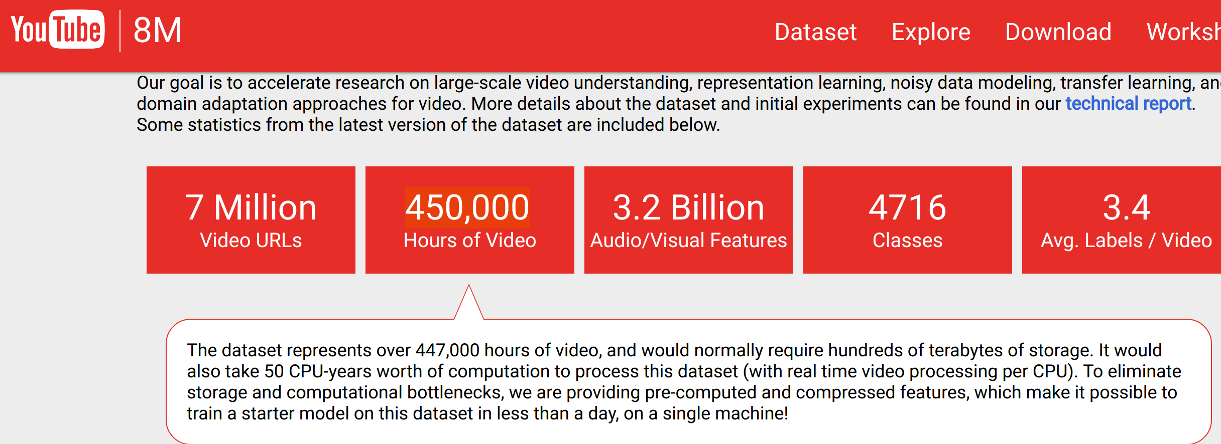
Feature counts:
Tables of word counts for documents.
Distributed by HathiTrust, JStor, etc.
For books, feature counts can be long!
Hathi EF is several TB.
Bridging the infrastructure for tokenization with the infrastructure for metadata.
Or: how can we distribute word counts as part of metadata profiles?
Prediction: Short, computer-readable embeddings of collections items will be an increasingly important shared resource for non-consumptive digital scholarship.
Embeddings promote access by opening new interfaces and forms of discoverability.
But embeddings deny access to classes of artifacts and communities that don't resemble their training set.
What's the best way to reduce dimensionality?
- Principal Components Analysis on the Term-Document matrix
- Latent Semantic Indexing
- Semantic Hashing, etc.
How do we reduce dimensionality?
- PCA on the words we can count.
- Top-n words.
- Topic models.
Reasons not to use the best methods.
- Computationally intractable: full matrix is trillions of rows, sparse matrix is billions.
- Difficult to distribute; users at home can't embed documents in your space.
- Any embedded space is optimal only for the text collection it was trained on.
A Minimal, Universal Dimensionality Reduction for text should:
- Be domain-agnostic.
- Be language-agnostic.
- Be capable of accounting for any vocabulary.
- Make only general assumptions about human language.
- Be capable of working from existing feature-count datasets.
- Be Easily implementable across platforms and languages.
Costs
- Inefficient use of dimensions (like top words).
- Dimensions cannot be cognizable, social things.
Costs
- Inefficient use of dimensions (like top words).
- Dimensions cannot be cognizable, social things.
Benefits
- Trivially parallelizable
- Allows client-server interactions
- preserving privacy/copyright concerns
- Reducing footprints
- Allows different corpora to exist in same space.
- Identifying duplicates
- Metadata extensions.
- Makes large datasets accessible for pedagogy.
2. Stable Random Projection.
Minimal, Universal reductions
- MinHash?
- The high-dimensional "Hashing Trick"
- Locality-sensitive hashing
Classic dimensionality reduction (pca, etc).
Starts with a document with W words.
For each word, learn an N-dimensional representation.
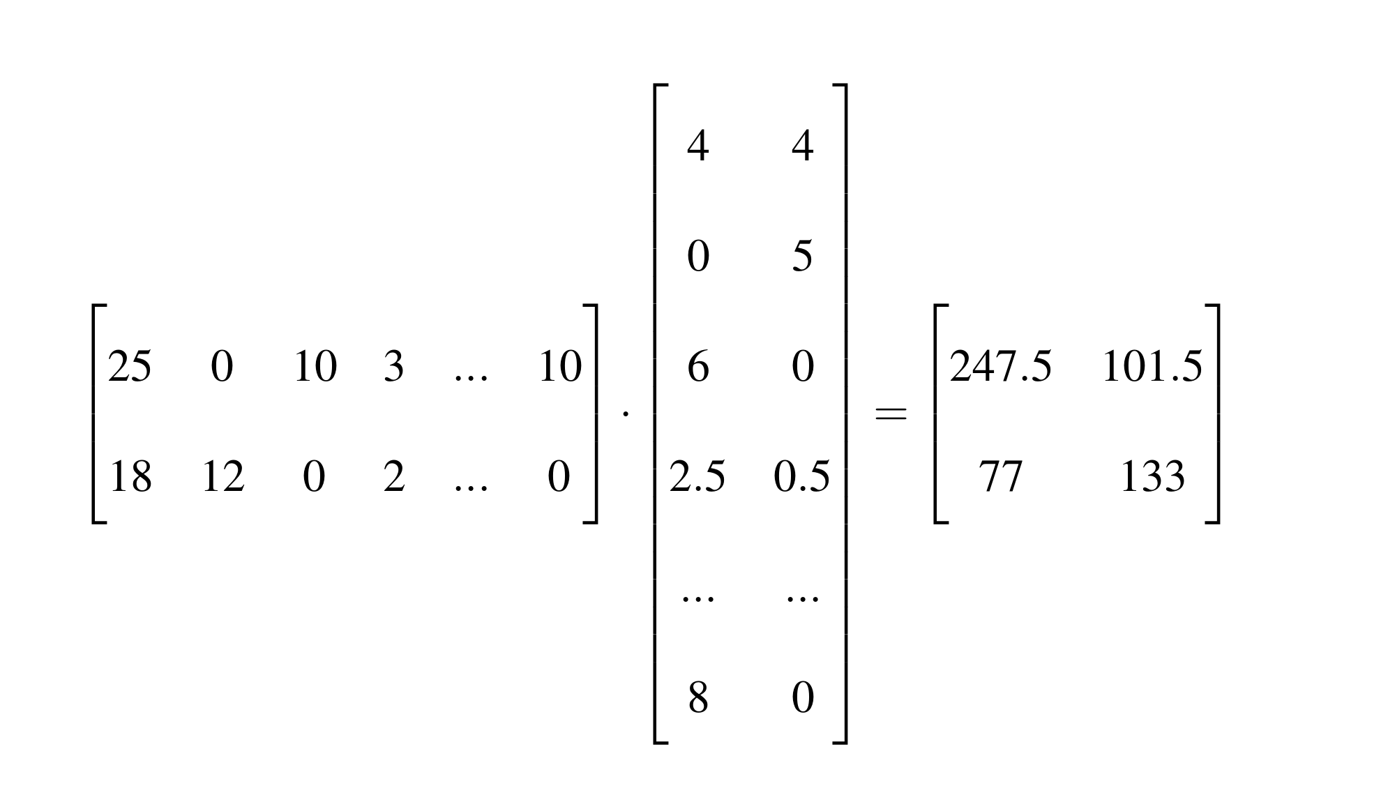
Multiple the document vector by a WxN matrix to get a N-dimensional representation of the document.
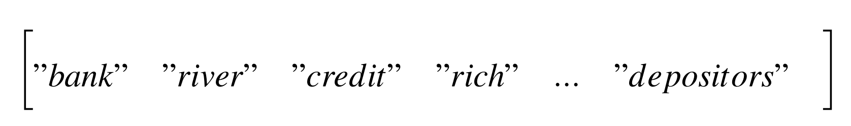
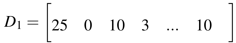
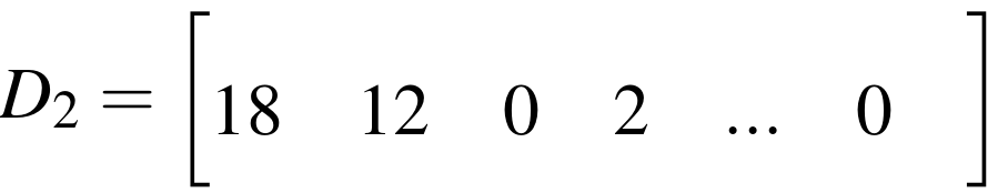
Example: Wordcounts
Example: word weights
Example: projection
SRP steps
- Begin with wordcounts
SRP steps
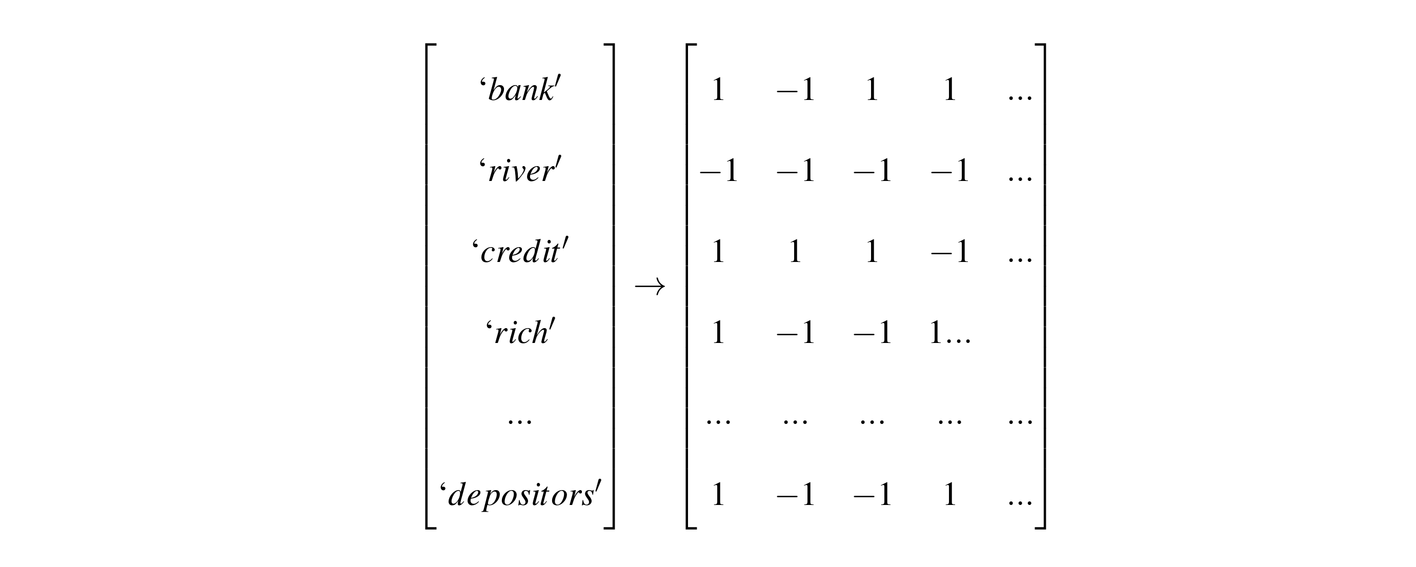
- Take SHA-1 hashes for all words.
(Because SHA-1 is available everywhere).
eg: "bank"
bdd240c8fe7174e6ac1cfdd5282de76eb7ad68151011110111010010010000001100100011111110011100010111010011100110101
0110000011100111111011101010100101000001011011110011101101110101101
1110101101011010000001010111101101010000011110100111110111000101001
01101111100111110000100111101100010101101101101110101101101010SRP steps
Cast the binary hash to [1, -1], (Achlioptas) generating a reproducible quasi-random projection matrix that will retain document-wise distances in the reduced space.
Put formally
D = Document, i = SRP dimension, W = Vocab size, h = binary SHA hash, w = list of vocabulary, c = counts of vocabulary.
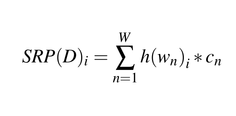
Put informally.
- Each dimension is the sum of the wordcounts for a random half the words, minus the sum of the wordcounts for the other half.
- Words that have the similar vocabulary will be closer on all the dimensions.
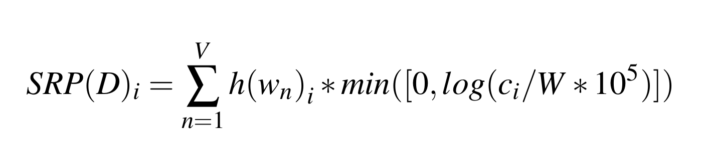
A final trick
Word counts are log transformed so common words don't overwhelm dimensions.
Denny/Spirling preprocessing.
Text Preprocessing For Unsupervised Learning: Why It Matters, When It Misleads, And What To Do About I
Hundreds of ways of pre-processing
Preprocessing for minimal dimensionality reduction.
Regularize as far as possible without making language-specific assumptions.
Do:
- Remove punctuation
- Lowercase.
- Replace numeric digits with '#'
Preprocessing for minimal dimensionality reduction.
Regularize as far as possible without making language-specific assumptions.
Don't:
- Lemmatize
- Remove stopwords
- Remove infrequent words
- Use bigrams.
Tokenization
One tokenization rule: unicode \w+.
"Francois doesn't have $100.00" ->
["francois","doesn","t","have","###","##"]`
One tokenization rule: unicode \w+.
Catastrophically bad for languages without whitespace tokenization!
Chinese, Thai, and some Devangari languages.
Unicode code-point based rules might be necessary--vowel splitting in Thai, character shingles in Chinese, etc.
.
3. Uses of the shared space.
Classification accuracy on Underwood/Sellars dataset.
Duplicate Detection
Classifier suites:
Re-usable batch training code in TensorFlow.
One-hidden-layer neural networks can help transfer metadata between corpora.
Protocol: 90% training, 5% validation, 5% test.
Books only (no serials).
All languages at once.
Classifiers trained on Hathi metadata can predict:
- Language
- Authorship on top 1,000 authors with > 95% accuracy. (Too good to be true)
- Presence of multiple subject heading components (eg: '650z: Canada-- Quebec -- Montreal') with ~50% precision and ~30% recall.
- Year of publication for books with median errors ~ 4 years.
4. Learning Library Classifications
Library of Congress Classification
- Shelf locations of books.
- Widely used by research libraries in United States.
- ~220 "subclasses" at first level of resolution.
| Instances | Class name (randomly sampled from full population) |
|---|---|
| 461 | AI [Periodical] Indexes |
| 6986 | BD Speculative philosophy |
| 9311 | BJ Ethics |
| 40335 | DC [History of] France - Andorra - Monaco |
| 2738 | DJ [History of the] Netherlands (Holland) |
| 14928 | G GEOGRAPHY. ANTHROPOLOGY. RECREATION [General class] |
| 17353 | HN Social history and conditions. Social problems. Social reform |
| 4703 | JV Colonies and colonization. Emigration and immigration. International migration |
| 23 | KB Religious law in general. Comparative religious law. Jurisprudence |
| 5583 | LD [Education:] Individual institutions - United States |
| 3496 | NX Arts in general |
| 6222 | PF West Germanic languages |
| 68144 | PG Slavic languages and literatures. Baltic languages. Albanian language |
| 157246 | PQ French literature - Italian literature - Spanish literature - Portuguese literature |
| 6863 | RJ Pediatrics |
.
Accuracy by language
.
Model Interpretability
Guesses for the text of "Moby Dick"
| Class | Probability |
|---|---|
| PS American literature | 62.658% |
| PZ Fiction and juvenile belles lettres | 30.729% |
| G GEOGRAPHY. ANTHROPOLOGY. RECREATION | 5.385% |
| PR English literature | 1.074% |
Why is "Moby Dick" classed as PR?
| Top positive for class PR | Top negative for class PR |
|---|---|
| 0.300% out (538.0x) | -0.294% as (1741.0x) |
| 0.289% may (240.0x) | -0.292% air (143.0x) |
| 0.258% an (596.0x) | -0.277% american (34.0x) |
| 0.239% had (779.0x) | -0.277% its (376.0x) |
| 0.238% are (598.0x) | -0.250% cried (155.0x) |
| 0.226% at (1319.0x) | -0.246% right (151.0x) |
| 0.221% english (49.0x) | -0.241% i (2127.0x) |
| 0.210% till (122.0x) | -0.231% days (82.0x) |
| 0.209% blow (26.0x) | -0.227% around (38.0x) |
| 0.208% upon (566.0x) | -0.205% back (164.0x) |

Classifying dates
Classifying dates
Representing time as a ratchet;
To encode 1985 in the range 1980-1990: [0,0,0,0,0,1,1,1,1,1]

Classification of Lucretius.
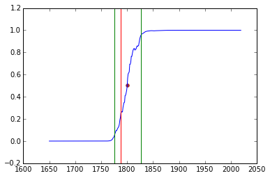
Blue line is classifier probability for each year Red vertical line is actual date. Outer bands are 90% confidence.